Day 1: Basic Mapping in R

1 Introduction

The goal for this session is to get you started with using RStudio, and being familiar with its environment. The session aims to introduce you to the basic programming etiquette, as well as building confidence for using RStudio as a GIS tool. At the end of this session, you should be able to perform some basic data managing tasks as well as generate a choropleth map in RStudio.

1.1 Learning outcomes

The first task includes becoming familiar with its environment and panels. We will begin a soft introduction on the basics of managing data in RStudio. This includes learning how to create various objects in RStudio such as vector and data frame objects. The crucial part of this session we be to know how to the set working directories as well as import your dataset in RStudio. Finally, we will learn how to perform the basic visualisation of spatial data in RStudio.

Let us begin.

1.2 Becoming familiar with the panels in RStudio

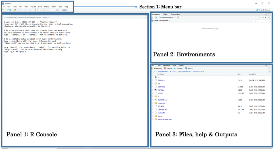
You should by now have opened RStudio on your laptop. When opening RStudio for the first time, you are greeted with its interface. The window is split into three panels: 1.) R Console, 2.) Environments and 3.) Files, help & Output.

Panel 1: The Console lets the user type in R-codes to perform quick commands and basic calculations.
Panel 2: The Environments lets the user see which datasets, spatial objects and other files are currently stored in RStudio’s memory
Panel 3: Under the File tab, it lets the user access other folders stored in the computer to open datasets. Under the Help tab, it also allows the user to view the help menu for codes and commands. Finally, under the Plots tab, the user can perusal his/her generated plots (e.g., histogram, scatterplot, maps etc.).

The above section is the Menu Bar. You can access other functions for saving, editing, and opening a new Script File for writing codes. Opening a new Script File will reveal a fourth panel above the Console.

You can open a Script File by:

Clicking on the File tab listed inside the Menu Bar. A scroll down bar will reveal itself. Here, you can scroll to the section that says New File.
Under New File, click on R Script. This should open a new Script File titled “Untitled 1”.

1.3 Using R Console as a Calculator

The R console window (i.e., Panel 1) is the place where RStudio is waiting for you to tell it what to do. It will show the code you have commanded RStudio to execute, and it will also show the results from that command. You can type the commands directly into the window for execution as well.

Let us start by using the console window as a basic calculator for typing in addition (+), subtraction (-), multiplication (*), division (/), exponents (^) and performing other complex sums.

Click inside the R Console window and type 19+8, and press enter key button ↵ to get your answer. Quickly perform the following maths by typing them inside the R Console window:

# Perform addition
19+8

# Perform subtraction
20-89

# Perform multiplication
18*20

# Perform division
27/3

# To number to a power e.g., 2 raise to the power of 8
2^8

# Perform complex sums
(5*(170-3.405)/91)+1002

Aside from basic arithmetic operations, we can use some basic mathematical functions such as the exponential and logarithms:

exp() is the exponential function
log() is the logarithmic function

These are quite useful functions for transforming or for standardising variables. You can perform the following execution of exp() and log() by typing them inside the R Console window:

# use exp() to apply an exponential to a value
exp(5) 

# use log() to transforrm a value on to a logarithm scale
log(3)

1.4 Creating basic objects and assigning values to it

Now that we are familiar with using the console as a calculator. Let us build from this and learn one of the most important codes in R programming called the Assignment Operator.

This arrow symbol <- is called the Assignment Operator. It is typed by pressing the less than symbol key < followed by the hyphen symbol key -. It allows the user to assign values or entire data structure(s) to an Object.

Objects are defined as stored quantities in RStudio’s environment. These objects can be assigned anything from numeric values to character string values. For instance, say we want to create a numeric object called x and assign it with a value of 3. We do this by typing x <- 3. When you enter the object x in the console and press enter ↵, it will return the numeric value 3.

Another example, suppose we want to create a string object called y and assign it with some text "Hello!". We do this typing y <- "Hello!". When you enter y in console, it will return the text value Hello.

Let us create the objects a,b, c, and d and assign them with numeric values. Perform the following by typing them inside the R Console window:

# Create an object called 'a' and assign the value 17 to it
a <- 17
# Type the object 'a' in console as a command to return value 17
a

# Create an object called 'b' and assign the value 10 to it
b <- 10
# Type the object 'b' in console as a command to return value 10
b

# Create an object called 'c' and assign the value 9 to it
c <- 9
# Type the object 'c' in console as a command to return value 9
c

# Create an object called 'd' and assign the value 8 to it
d <- 8
# Type the object 'd' in console as a command to return value 8
d

Notice how the objects a, b, c and d and its value are stored in RStudio’s environment panel. We can perform the following arithmetic operations with these object values:

# type the following and return an answer
(a + b + c + d)/5

# type the following and return an answer
(5*(a-c)/d)^2

Let us create more objects but this time we will assign character string(s) to them. Please note that when typing a string of characters as data you will need to cover them with quotation marks "...". For example, say we want to create a string object called y and assign it with some text "Hello!". We do this by typing y <- "Hello!".

Try these examples of assigning the following character text to an object:

# Create an object called 'e' and assign the character string "RStudio"
e <- "RStudio"
# Type the object 'e' in the console as a command to return "RStudio"
e

# Create an object called 'f', assign character string "Hello world" 
f <- "Hello world"

# Type the object 'f' in the console as a command to return "Hello world"
f

# Create an object called 'g' and assign "Blade Runner is amazing"
g <- "Blade Runner is amazing"
# Type the object 'g' in the console to return the result
g

We are now familiar with using the console and assigning values (i.e., numeric and string values) to objects. The parts covered here are the initial steps and building blocks for coding and creating datasets in RStudio.

Let us progress to the next section. Here is where the serious stuff start. We will learn the basics of managing data and some coding etiquette - this includes creating data frames, importing & exporting spreadsheets, setting up work directories, column manipulations and merging two data frames. Learning these basic tasks are key for managing data in R/RStudio.

Important

Point of no return: From here on out - let us open a script file and type codes there instead of the Console! We are getting serious now, we will never use the Console again.

2 Basics of managing data in RStudio

2.1 How do we enter data into RStudio?

As you have already seen, RStudio is an object-oriented software package and so entering data is slightly different for the usual way of inputting information into a spreadsheet (e.g., Microsoft Excel). Here, you will need to enter the information as a Vector object before combining them into a Data Frame object.

Consider this crude example of data containing the additional health information for 4 people. It contains the variable (or column) names ‘id’, ‘name’, ‘height’, ‘weight’ and ‘gender’

id	name	height	weight	gender
1	Kofi	1.65	64.2	M
2	Harry	1.77	80.3	M
3	Huijun	1.70	58.7	F
4	Fatima	1.68	75.0	F

Now, when entering data to RStudio it is not like Microsoft Excel where we enter data into the cells of a spreadsheet. In RStudio, data is entered as a sequence of elements and listed inside an object called a vector. For instance, if we have three age values of 12, 57 and 26 years, and we want to enter this in RStudio, we need to use the combine function c() and combine these three elements into a vector object. Hence, the code will be c(12, 57, 26). We can assign this data by typing this code as age <- c(12, 57, 26). Any time you type ‘age’ into RStudio console it will hence return these three values unless you chose to overwrite it with different information.

Let us look at this more closely with the 'id' variable in the above data. Each person has an ID number from 1 to 4. We are going to list the numbers 1, 2, 3 and 4 as a sequence of elements into a vector using the combine function c() and then assign it to as a vector object calling it 'id'.

# Create 'id' vector object 
id <- c(1, 2, 3, 4)

# Type the vector object 'id' in console to see output
id

Now, let us enter the information the same way for the remaining columns for ‘name’, ‘height’, ‘weight’ and ‘gender’ like we did for ‘id’:

# Create 'name' vector object
name <- c("Kofi", "Harry", "Huijun", "Fatima")

# Create 'height' (in meters) vector object
height <- c(1.65, 1.77, 1.70, 1.68)

# Create 'weight' (in kg) vector object
weight <- c(64.2, 80.3, 58.7, 75.0)

# Create 'gender' vector object
gender <- c("M", "M", "F", "F")

Now, that we have the vector objects ready. Let us bring them together to create a proper dataset. This new object is called a Data frame. We need to list the vectors inside the data.frame() function.

# Create a dataset (data frame)
dataset <- data.frame(id, name, height, weight, gender)

# Type the data frame object 'dataset' in console to see output
dataset

# You can also see dataset in a data viewer, type View() to data:
View(dataset)

Note

The column ‘id’ is a numeric variable with integers. The second column ‘name’ is a text variable with strings. The third & fourth columns ‘height’ and ‘weight’ are examples of numeric variables with real numbers with continuous measures. The variable ‘gender’ is a text variable with strings – however, this type of variable is classed as a categorical variable as individuals were categorised as either ‘M’ and ‘F’.

2.2 How do we create a variable based on other existing variables in our data frame?

To access a variable by its name within a data frame, you will need to first type the name of the data frame followed by a $ (dollar sign), and then typing the variable’s name of interest. For instance, suppose you just want to see the height values in the Console viewer - you just type:

# to access height - you need to type 'dataset$height'
dataset$height

We can use other columns or variables within our data frame to create another variable. This technique is essentially important when cleaning and managing data. From this dataset, it is possible to derive the body mass index bmi from height and weight using the formula:

$BMI = weight/height^2$

To generate bmi into our data frame, we would need to access the height (m) and weight (kg) columns using the $ from the data frame its stored to, and apply the above formula as a code to generate the new bmi column:

# Create 'bmi' in the data frame i.e.,'dataset' and calculate 'bmi'
# using the $weight and $height
dataset$bmi <- dataset$weight/((dataset$height)^2)
# View the data frame ‘dataset’ and you will see the new bmi variable inside
View(dataset)

You can overwrite the height (m) column to change its units into centimeters by multiplying it to 100; equally, the weight (kg) column can be overwritten and converted from units of kilograms to grams by multiplying it to 1000.

# using $height and *100 
dataset$height <- dataset$height*100
# using $weight and *100
dataset$weight <- dataset$weight*1000
# use View() the data frame ‘dataset’ and you will see the updated variables
View(dataset)

2.3 How do we set the working directory in our computer by connecting our folder to RStudio with the `setwd()` function?

Now, we are getting very serious here!

Important

Before we do anything - make sure to have downloaded the data set for this session if you haven’t done so by clicking here. In your computer, create a new folder on your desktop page and rename the folder to “BISemWeb2025”, and create another folder within “BISemWeb2025” and rename it as “Day 1”. Make sure to unzip and transfer ALL the downloaded data directly to the Day 1 folder.

Now, this part of the practicals are probably the most important section of this tutorial. It’s usually the “make” or “break” phase (i.e., you will either end-up loving RStudio OR you will end-up hating it and not ever wanting to pick up R again!).

We are going to learn how to set-up a working directory. This basically refers to us connecting the RStudio software to the folder containing our dataset. It allows the user to tell RStudio to open data from a folder once it knows the path location. The path location specifies the whereabouts of the data file(s) stored within a computer. Setting your directory in RStudio beforehand makes life incredibly easier in terms of finding, importing, exporting and saving data in and out of RStudio.

To illustrate what a path location is – suppose on my desktop (mac/windows) there is a folder called “BISemWeb2025”, and within that folder, exists another folder called “Day 1”. Finally, suppose a comma separated value (.csv) data file called “CIV_Sub_Prefecture_Mosquito_Data.csv” is stored in it (i.e., Day 1). If via RStudio you want to open this CSV data file located in within the “Day 1” folder. You will need to first set the path to the “Day 1” folder in RStudio using the setwd() function.

Therefore, the path location to this folder on a Windows machine would be written as follows, "C:/Users/accountName/Desktop/BISemWeb2025/Day 1". You can access this piece of information simply by:

Open the BISemWeb2025 folder to reveal the Day 1 folder.
Open the Day 1 folder in the data files are stored.
Now, click on the bar at the top which shows BISemWeb2025 > Day 1. This should highlight and show "C:\Users\accountName\Desktop\BISemWeb2025\Day 1" (see image below):

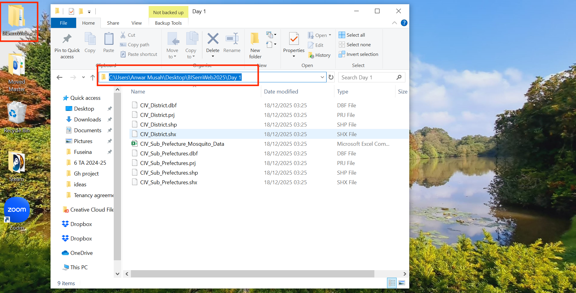
Now, copy "C:\Users\accountName\Desktop\BISemWeb2025\Day 1" and paste the path name into the setwd() function in your R script.
Lastly, change all the back slashes \ in the path name to forward slashes / and run the code. It should look like this: setwd("C:/Users/accountName/Desktop/BISemWeb2025/Day 1").

For Windows, the setwd() is as follows:

# set work directory in windows
setwd("C:/Users/accountName/Desktop/BISemWeb2025/Day 1")

For MAC users, its marginally different. The path location would be written as follows, "/Users/accountName/Desktop/BISemWeb2025/Day 1". You can access this piece of information simply by:

Right-clicking on the folder “Week 1” (not file) in which the files are stored.
Hold the “Option” ⌥ key down

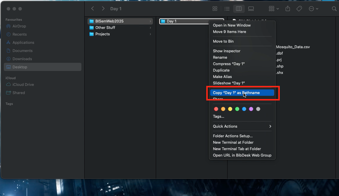
Click Copy "filename" as Pathname
Paste the copied path name into the function setwd() and run the code

For Mac, the setwd() is as follows:

# set work directory in macs
setwd("/Users/accountName/Desktop/BISemWeb2025/Day 1")

This should set the working directory. Now, let us learn how to import a CSV data into RStudio.

2.4 How do we import a CSV data in RStudio?

As you will be working mostly with comma separated value formatted data (i.e., csv) we will therefore learn how to import and export in RStudio. There are three files (1 CSV, 2 shapefiles) that we are going to import into RStudio:

CIV_Sub_Prefecture_Mosquito_Data.csv which contains four columns about mosquito (i.e., Anopheles Gambiae) populations after insecticide campaign in Cote d’Ivoire across 113 sub-prefectures - NAME_3 (the name of sub-prefecture); TOTAL_MOSQ (total number of mosquitoes), TOTAL_MOSQ_DEATH (total number of mosquitoes that died after exposure to the insecticide), TOTAL_MOSQ_SURV (total number of mosquitoes that survived after exposure to the insecticide) and MORTALITY_ADJ_AVR (mortality adjusted rate).
CIV_District.shp which is a vector layer containing the spatial boundaries of the 14 districts in Cote d’Ivoire.
CIV_Sub_Prefectures.shp which is a vector layer containing the spatial boundaries of the 113 sub-prefectures in Cote d’Ivoire.

To import a csv into RStudio, we use the read.csv() function. To demonstrate this, let us import the data for fires into an data frame object and name it as CIV_Agg_Insect_ADMIN3

# Import data using read.csv() function 
CIV_Agg_Insect_ADMIN3 <- read.csv(file = "CIV_Sub_Prefecture_Mosquito_Data.csv", header = TRUE, sep = ",")

Important

The arguments used in read.csv() function – 1.) ‘file =’ is a mandatory option where you quote the name of the file to be imported; 2.) ‘header = TRUE’ option is set to TRUE which is telling RStudio that the file that is about to be imported has column names on the first row so it should not treat as observations; and 3.) ‘sep = ","’ we are telling RStudio that the format of the dataset is comma separated.

We have imported the mosquito data. You can actually view the spreadsheet in the data viewer window using the code View():

# Show viewer the data set
View(CIV_Agg_Insect_ADMIN3)

2.5 How do we import a shapefile into RStudio?

2.5.1 Installing packages into RStudio

So far, we have been using functions and commands that are by default native or built-in RStudio. As you will become more and more proficient in RStudio, you will come to realise that there are several functions in RStudio that are in fact not built-in by default which will require external installation.

For instance, the sf package which is called Simply Features allows the user to load shapefiles (a type of Vector spatial data) into RStudio’s memory. Another important package is called tmap, this package gives access to various functions that allows the user to write code and emulate RStudio as a GIS software. These are examples of packages with enables mapping of spatial data. They need to be installed as they not built-in programs in RStudio.

Let us install following packages: tmap and sf using the install.packages() function, and then initiate the packages to make them active in RStudio using the library() function.

First sf and tmap packages:

install.packages("sf")
install.packages("tmap")

Once the installation is complete, you MUST activate the packages using the library() function. Type the following to perform this action:

# Active the sf and tmap packages
library("sf")
library("tmap")

2.5.2 Using the `read_sf()` to import shapefiles in RStudio

The sf package grants the user access to a function called read_sf() to read-in shapefiles into RStudio. A shapefile typically contains the geometry of the spatial features e.g., points, line segment and boundaries of an areal feature etc. The shapefile has the extension of .shp (and it is always accompanied by its other supporting files with extensions .shx, .prj, .dbf and .cpg).

Warning

The following files must all be stored in the same folder location with the .shp file (i.e., .shx, .prj, .dbf and .cpg). If one is missing - the .shp file will not work!

Recall, we have two shapefiles:

CIV_District.shp for the districts
CIV_Sub_Prefectures.shp for the sub-prefectures.

We can easily load them in RStudio as Spatial Polygon objects, type into your script:

# Add shapefiles
CIV_ADMIN1 <- read_sf("CIV_District.shp")
CIV_ADMIN3 <- read_sf("CIV_Sub_Prefectures.shp")

2.5.3 Joining two datasets by merger using the `merge()` function

You will often find yourself merging two or more data frames together, especially bringing together a spatial object with a non-spatial object. We cannot stress the importance of merging objects in the correct order so that the spatial attributes are preserved.

In this instance, we are just dealing with non-spatial dataset - i.e., the object CIV_Agg_Insect_ADMIN3 because while it contain the prefecture names it does not contain the geometry of those areas.

However, the object CIV_ADMIN3 is a spatial dataset - as it contains the geometries that define the polygons of sub-prefecture areas (see image).

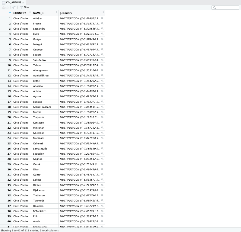
You can also check this by using the View() function on CIV_ADMIN3:

View(CIV_ADMIN3)

We need merge these two objects CIV_ADMIN3 & CIV_Agg_Insect_ADMIN3using the merge() function. Consequently, we want the format of the merge code to look something akin to this syntax merge(target_object, selected_object, by="NAME_OF_LINK_COLUMN").

Merging data frames is indeed a very important technique to know especially if you need to bring together event information with no spatial dimension with actual spatial data for it to be mappable.

Alright, let’s merge the mosquito data using the NAME_3 column with the shapefile dataset:

# Merge the non-spatial table with ADMIN3 data frame
CIV_Spatial_Data <- merge(CIV_ADMIN3, CIV_Agg_Insect_ADMIN3, by.x = "NAME_3", by.y = "NAME_3", all.x = TRUE)
# View the datasets
View(CIV_Spatial_Data)

Important

The arguments used in merge.csv():

CIV_ADMIN3 is the target data frame we want something to be merged on to.
CIV_Agg_Insect_ADMIN3 is the selected data frame we are using to merge with the CIV_ADMIN3.
by.x = "NAME_3" option we are specifying the name of the join column from the target data frame i.e., CIV_ADMIN3.
by.y = "NAME_3" option we are specifying the name of the join column from the selected data frame i.e., CIV_Agg_Insect_ADMIN3
all.x=TRUE option we are telling RStudio to retain all rows that are originally from the target data after merging regardless of whether or not they are present in the selected data frame. So even if a row from the selected data does not find a unique link with any of the rows in the target data to match - it will still preserve the target data frame by not discarding unlinked rows. But it will discard the unmatched rows from the selected data frame.

3 Basic visualisation of spatial data in RStudio

3.1 Mapping with ‘tmap’ functions in RStudio

The tmap is the best package for creating maps in RStudio – it’s easy to code and user friendly. Let’s finally start some mapping! Here are some basic ‘tmap’ functions to be very familiar with:

`tmap` functions	What it does…
`tm_shape()`	This allows the user to add layers to be mapped
`tm_polygons()`	This deal with vector type dataset specifically. This allows the user to specify which column in the vector layer to be mapped using the `fill =` argument. Within the `tm_polygon()`, it also allows the user to apply the appropriate customisation to the vector layer. Examples of such arguments in 1.) `fill_alpha =` to modify the transparency; 2.) `col_alpha =` to modify the transparency of the borders; 3.) `col =` controls the colour of the line; 4.) `fill.scale =` controls the appearence and set the colour scheme of the scale that appears inside the legends block. Please note that if your data is continuous, then the appropriate argument to use in the `fill.scale =` would be either `tm_scale_continuous()` or `tm_scale_interval()` for breaking the continuous values into intervals. If they are numerical but discrete (counts) use `tm_scale_discrete()`. Otherwise, if it is categorical use `tm_scale_categorical()`; and 4.) `fill.legend = tm_legend(...)` allows the user to control the presentation of the legend. There are many arguments to experiment with - you can type `?tm_polygons()` in console to see them. Please note that the `tm_polygons()` is immediately followed after specifying the `tm_shape()` function.
`tm_layout()`	This allows the user to make heavy customisations to the main title, legends and other cosmetics to text sizes etc.
`tm_compass()`	This allows the user to add a compass visual to the map output
`tm_scale_bar()`	This allows the user to add a scale bar to the map output

3.1.1 Visualising the outline(s) of study area

Suppose you want to visual just the outline of Cote d’Ivoire’s prefecture areas only:

# Visual outline of prefecture only
tm_shape(CIV_Spatial_Data) + tm_polygons()

We use the function tm_shape() and insert the CIV_Spatial_Data spatial object into its function, since we are plotting polygons follow it up with the function tm_polygons()

Note

Note that the above example is applies no customisation to the map!

You can customise the level of transparency for both the area and borders by adding some arguments in the tm_polygon() [i.e., fill_alpha, and col_alpha which only take values between 0 (full transparency) to 1 (100% solid)]. fill_alpha controls the transparency of the areas, and col_alpha controls the transparency of the borders.

For example:

tm_shape(CIV_Spatial_Data) + tm_polygons(fill_alpha = 0.1, col_alpha = 0.4)

3.1.2 Adding another layer on top of study area

Suppose you want to add another layer to show the regions (i.e., Districts) of Cote d’Ivoire for which the sub-prefecture areas reside in, you can use another tm_shape() in the code add that additional layer, the coding would be as follows:

# Adding another layer

tm_shape(CIV_Spatial_Data) + 
    tm_polygons(fill_alpha = 0.1, col_alpha = 0.4) +
tm_shape(CIV_ADMIN1) +
    tm_polygons(fill_alpha = 0, col_alpha = 1, col = "black", lwd = 2)

# The background of the added layer (CIV_ADMIN1) has been rendered to full transparency with the fill_alpha set to 0 and it borders are fully solid using col_alpha set to 1 and col (colour) set to “black” to appear pronounced. In addition, we have thickened the line by using setting that controls the line thickness `lwd = 2`

3.1.3 Full visualising of data in the maps

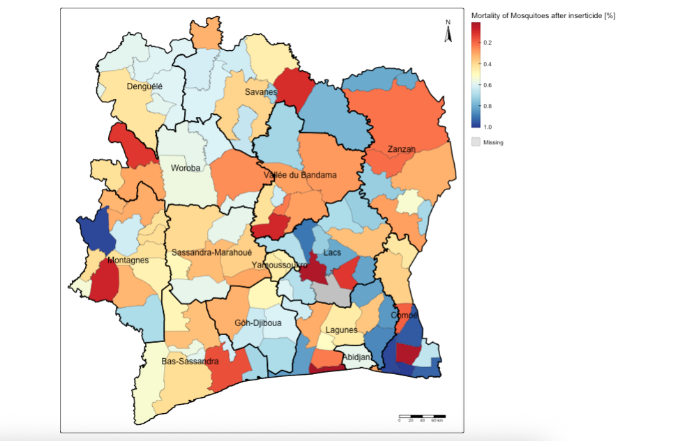
Suppose you want to visualise the spatial data in sub-prefectures, we can use the tm_polygons() function to specify the column of interest. For instance, let us visual the MORTALITY_ADJ_AVR column which has CONTINUOUS (or proportion) values ranging from 0 to 1 to signify areas that successfully reduced the treat of mosquito populations through insecticide application (with 1 equivalent to 100% mortality of mosquitoes after being exposed to the insecticide) and vice versa (with 0 meaning that all mosquitoes survived indicating resistance to this insecticide).

The coding would be as follows:

# full visualisation
tm_shape(CIV_Spatial_Data) + 
    tm_polygons(
        fill = "MORTALITY_ADJ_AVR",
        fill.scale = tm_scale_continuous(values = "brewer.rd_yl_bu"),
        fill.legend = tm_legend(title = "Mortality of Mosquitoes after inserticide [%]", frame = FALSE, position = tm_pos_out()),
        fill_alpha = 1, col_alpha = 0.5, col = "black", lwd = 0.5) +
tm_shape(CIV_ADMIN1) + tm_text("NAME_1") +
    tm_polygons(fill_alpha = 0, col_alpha = 1, col = "black", lwd = 2) +
tm_compass(type = "arrow", position = c("right", "top")) +
tm_scalebar(position = c("right", "bottom"))

In the tm_polygons(), we insert the variable of interest we want to visual at the fill = argument. The fill.scale = option allows us to select the appropriate fill scale colour scheme depending on the type of dataset we are using - here it is continuous, so we use tm_scale_continuous(). The fill_legend() allows us to apply the appropriate customisation to the legends in the legend block.

You can also check all the available list of colour schemes by typing the code: cols4all::c4a_palettes().

Note

Geography 101 – when creating a map, it is always best to add the North compass and scale bar. This is done with the tm_compass() and tm_scalebar() functions. The tm_layout() allows you to make further customisations to the internal and external plot region of map such as turning of the plot frame or modifying the text size in output. You can experiment with them by checking the help menu – just type: ?tm_layout() in the console.

3.2 Generating interactive maps

By running the code: tmap_mode("view"), will cause all map outputs to be generated in interactivity mode.

tmap_mode("view")

This should switch the plot from being static to something that is now dynamic. If we run code to generate the full map again, it will be displayed as an interactive map:

tm_shape(CIV_Spatial_Data) + 
    tm_polygons(
        fill = "MORTALITY_ADJ_AVR",
        fill.scale = tm_scale_continuous(values = "brewer.rd_yl_bu"),
        fill.legend = tm_legend(title = "Mortality of Mosquitoes after inserticide [%]", frame = FALSE, position = tm_pos_out()),
        fill_alpha = 1, col_alpha = 0.5, col = "black", lwd = 0.5) +
tm_shape(CIV_ADMIN1) + tm_text("NAME_1") +
    tm_polygons(fill_alpha = 0, col_alpha = 1, col = "black", lwd = 2) +
tm_compass(type = "arrow", position = c("right", "top")) +
tm_scalebar(position = c("right", "bottom"))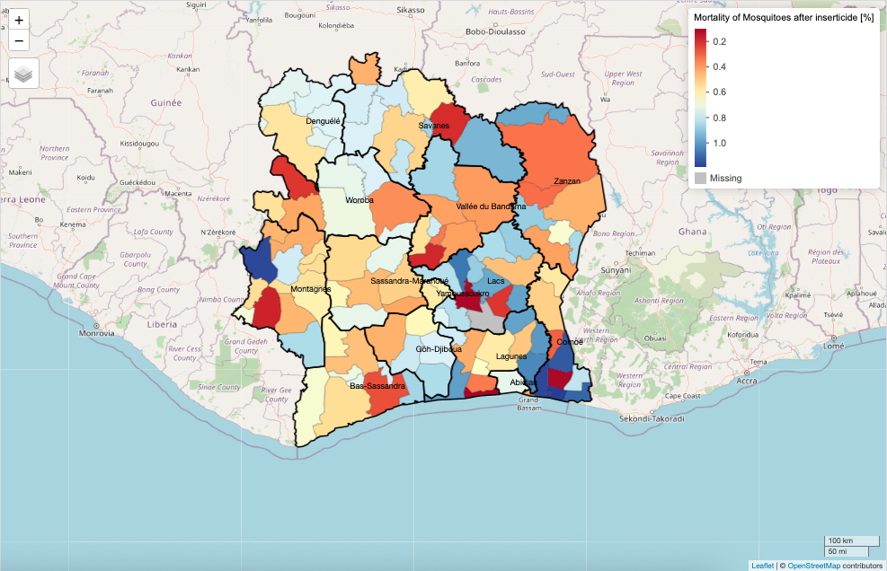

You can switch it off by running the following code: tmap_mode("plot") to revert it back to static mode.

tmap_mode("plot")

This concludes Day 1’s session. On Day 2, we will use same the dataset to see if there is any patterns of clustering on where mosquitoes thrive despite being exposed to insecticides.

4 Data Sources

Malaria Threat Map (see: “Vector Insecticide Resistance”)[Source: World Health Organisation (WHO)] Click Here
Shapefiles for Cote d’Ivoire [Source: Database of Global Adminstrative Areas (GADM)] Click Here

Warning

IMPORTANT NOTE: Users should be aware that the original data used in this practical were obtained from WHO’s Malaria Threat Map (Vector Insecticide Resistance). The dataset consists of survey point locations of mosquito occupancy (total) for Anopheles species exposed to insecticides, including counts of mosquitoes that survived and those that died.

For the purposes of this practical and to visualise area-level information, these point-level measures were aggregated to the sub-prefecture level. To complete the dataset for sub-prefectures with missing data, the aggregated data were resampled using Bayesian methods, incorporating information from neighbouring areas to fill in the gaps.

1 Introduction

1.1 Learning outcomes

1.2 Becoming familiar with the panels in RStudio

1.3 Using R Console as a Calculator

1.4 Creating basic objects and assigning values to it

2 Basics of managing data in RStudio

2.1 How do we enter data into RStudio?

2.2 How do we create a variable based on other existing variables in our data frame?

2.3 How do we set the working directory in our computer by connecting our folder to RStudio with the setwd() function?

2.4 How do we import a CSV data in RStudio?

2.5 How do we import a shapefile into RStudio?

2.5.1 Installing packages into RStudio

2.5.2 Using the read_sf() to import shapefiles in RStudio

2.5.3 Joining two datasets by merger using the merge() function

3 Basic visualisation of spatial data in RStudio

3.1 Mapping with ‘tmap’ functions in RStudio

3.1.1 Visualising the outline(s) of study area

3.1.2 Adding another layer on top of study area

3.1.3 Full visualising of data in the maps

3.2 Generating interactive maps

4 Data Sources

2.3 How do we set the working directory in our computer by connecting our folder to RStudio with the `setwd()` function?

2.5.2 Using the `read_sf()` to import shapefiles in RStudio

2.5.3 Joining two datasets by merger using the `merge()` function