Part 3: Exploratory analysis in RStudio
What is statistics and data in general?
Definition 1: Statistics is a branch in the mathematical sciences that pertains to the collection, analysis, interpretation, and graphical presentation of data. The best thing about statistics is that it’s a highly applied branch of science which is applicable to many areas such as social science, politics, health (e.g., epidemiology), business & finance, environmental sciences and geography.
Statistics is broadly split into two main areas:
- Descriptive statistics, which focuses on describing the visible characteristics about a dataset
- Inferential statistics is more research-based, which focuses on making predictions (rather than stating facts) and testing hypothesis about a phenomenon.
Definition 2: A variable is any characteristics, numbered value, or quantity that can be measured or counted. A variable can also be referred to a data Item. A variable can be broadly classified as discrete, continuous or categorical variable.
We have provided two videos: the first which broadly explains why statistics as a subject is important; and the second explains in much details what statistics is as a subject, and what are the various data types.
[Theory] Why is statistics important? (Length: 13:21 minutes)
Watch on YouTube [LINK]
[Theory & Code] What is statistics, and the types of variables? (Length: 31:17 minutes)
Watch on YouTube [LINK]
Analysing air pollution data in Barcelona
We will focus on descriptive statistics as an introduction introducing everyone to the absolute basics. Descriptive statistics is all about knowing the data types and finding the distribution, central tendency and variability in such data set. These four key words may sound intimidating – but trust me – it is very easy! Let us learn how to perform this in RStudio using the air pollution data for Barcelona.
Let us import for following dataset Barcelona_Air_Pollution_data.csv into RStudio, and call this object air_ quality_data.
Remember - always make sure that your work directory is linked to your folder containing your data.
For Windows:
For Macs:
Now, import you the data set as follows:
You use the command View() see the full data viewer, or head() to see the first five rows of the dataset.
You will notice that the data contains six variables with the following information:
| Variable name | Variable Type | Information |
|---|---|---|
| Location | String/Text only | Name of location Eixample, Barcelona |
| ReadingDate | Date | Data collection date for air quality measures |
| NO2_est | Continuous | Measurements for Nitrogen dioxide (NO\(_2\)) (ppb) |
| NO2_category | Categorical | Health impacts (negligible/low/moderate/high) |
| PM10_est | Continuous | Measurements for Particulate matter (PM10) |
| PM10_category | Categorical | Health impacts (negligible/low/moderate) |
Important Notes: The NO2_est, for example, contains measurable items i.e., 718 observations for concentrations of ambient NO\(_2\) in Eixample area of Barcelona, and hence its a continuous variable. These estimates have been categorised in accordance with their health dangers i.e., negligible (\(<\) 10 ppb); low (11-50 ppb); moderate (51-100 ppb) and high (>101 pbb). The categories are contained in the variable NO2_category.
Let us begin to analyse NO2_est and NO2_category with frequency distributions
Frequency distributions
We use frequency distribution to analyse a set continuous data. In data handling in this context, there are two outputs generated:
- Frequency, which tells us how often a particular result was obtained. From this we can calculate a percentage value which is referred to as Relative Frequency.
- Cumulative Frequency, this is a cumulative sum of the frequencies, which indicates how often a result was obtained that is less than a stated value in our collection of data. Again, from this we can also calculate a cumulative percentage value which is referred to as Cumulative Relative Frequency.
Suppose, we want to assess the 718 observations for air pollutant Nitrogen Dioxide (NO\(_2\)).
Let’s list the observations for Nitrogen Dioxide (NO\(_2\)) in Barcelona:
##   [1]  61  59  29  75  23  49  43  35  83  75  71  56  54  44  41  54  62  56
##  [19]  26  42  71  86  85  52  56  45  68  86  69  71   4  82  43  51 114  43
##  [37]  18  58  24  53  98  53 100  53  49  49  46  82  77  67  76  52  61  80
##  [55]  77  70  56  49  42  73  64  33  71  72  13  37  26  46  84  72  65  76
##  [73]  90  46  61  81  64  62  58  78  83  37 130  43  20  40 102  68  48  74
##  [91]  52  43  80  71  42  84  44 121  41  66  44  50  38  75  41  45  48  63
## [109]  53  63  63  46  34  87  75  74  36  69  46  15  80  75  83  95   5  65
## [127]  21  84  68  32  45  73  53  31  85  91  73  46  25  75  70  84  68  65
## [145]  58 113  62  60  55  69  82 100 105  47  60 103  53  34  39  22  21  71
## [163]  85  56  73  61  24  44  47  49 100  64  91  79  42  32  33  84  43  61
## [181]  63  49  80  46  58  45  37  66  60  75  35  75  48  43  57  67  54  38
## [199]  22  51  69  51  64  32  20  52  42  65  69  47  40  34  34  51  57  43
## [217]  52  86  53  43  54  75  56  62  41  84  41  22  83  76  51  31  50  65
## [235]  76  77  61  50  75  49  47  65  78  39  51  49  75  45  50  69  86  75
## [253]  89  68  84  90  90  56 106  63  90  57  38  86  22  39  19  61  44  63
## [271]  52  42  46  56  40  69  62  42  54  17  49  84  34  89  65  53  78  67
## [289]  55  61  39  82  58  15  63  76  55  80  56  79  72  58  74  27  93  40
## [307]  40  58  79  81 123  84  37  87  38  49  91  50  59  69  57  68  53  38
## [325]  51  78  71  72  55  70  56  63  85  78  64  23  84  43  46  33  59  58
## [343]  47  64  68  89  76  86 116  52  34  63  40  41  72  87  37  62  38  68
## [361]  88  39  59  77  75 112  44  40  90  37  66  61  65  50  79  79  36  36
## [379]  12  86  40  62  63  71  53  30  44  76  41  62  77  80  62  86  37  48
## [397]  80  55  56  49  84  48  49  84  60  76  28  77  41  57  55  51  54  54
## [415]  11  43  38  86  30  23  78  29  80  16  48  90  44  42  50  54  45  42
## [433]  70  49  67  73  60  42  99  97  77  46  52  24  75  30  70  81  53  17
## [451]  63  59  44  41  67  56  58 111  43  47  49  58  36  72  36 103  63  77
## [469]  65  42  42  79  41  24  59  50  46  55  77  91  54  70  73  53  80  53
## [487]  72  67  95  57  87  39  73  56  34  56  75  74  72  42 119  55  43  69
## [505]  55  52  77  63 108  43  61  47 117  80  61  67  78  49  42  35  58  54
## [523]  36  84  56  72  70  40  59  71  56  49  66  52  48  60  54  73  66  67
## [541]  70  93  65  60  13  83  49  42  62  63  50  46  54  94  73  54  74  54
## [559]  10  71  41  17  75  55  54  54  83  47  49  90  76  89  83  43  76  67
## [577]  75  88  59  60  34  36  63  42  59  71  73  73  40  74  53  56  99  46
## [595]  46  64  37  20  84  86  47  57  54  56  78  73  65  72  37  57  38  46
## [613]  43  57  98  32  98  53  86  59  63  42  60  60  51  58  59  83  67  42
## [631]  74  62  84  67  49  76   2  44  51  69  69  87  49  18  73  66  81  78
## [649]  82  69  50  36  71  60   7  50  49  60  55  25  58  76  69  61  88  45
## [667]  59  59  91  61  81  81  83  71 108  99  46  69  38  54  59  16  75  81
## [685]  35  63  65  71  57  53  58  37  39  43  64  76  56  72  87  74  74  77
## [703]  46  87  53  60  47  10  61  35  36  60  71  45  47  79  37 123
In a list format it is quite difficult to make head or tail on what observations appear frequently and its distribution. To summarise this - it will be helpful to classify the information into Classes and then obtain the Frequency and Cumulative Frequency in a table. We call this table a Frequency Table.
The minimum value for NO\(_2\) is 2 and the maximum is 130. We can group the 718 observations into 13 classes using an interval of 10s e.g., 1-10, 11-20, 21-30, 31-40, 41-50, 51-60, 61-70, 71-80, 81-90, 91-100, 101-110, 111-120 and 121-130
Important Notes: The way and manner you specify the classes and interval are up to you really. Here, 10 is being used for convenience.
The interval width is 10, we can generate sequence of number from 0 to 130, inclusively, to create the classes which in turn be used to group the 718 observations into 13 classes using the seq() and cut().
For example:
# using starting value as 0
# using highest value as 130
# using interval as 10

#  specify in this order the lower, highest, interval value in seq() function
classes <- seq(0, 130, 10)
classes
## [1] 0 10 20 30 40 50 60 70 80 90 100 110 120 130The sequence of values are stored in the object called classes. Now, let us apply the cut() function to group the NO\(_2\) data accordingly. We can do this by generating a new variable called Groups.
# tell the cut() function to group NO2_est using the classes object
air_quality_data$Groups <- cut(air_quality_data$NO2_est, breaks=classes)
air_quality_data$Groups
## [1] (60,70] (50,60] (20,30] (70,80] (20,30] (40,50] (40,50]
## [8] (30,40] (80,90] (70,80] (70,80] (50,60] (50,60] (40,50]
## [15] (40,50] (50,60] (60,70] (50,60] (20,30] (40,50] (70,80]
## [22] (80,90] (80,90] (50,60] (50,60] (40,50] (60,70] (80,90]
## [29] (60,70] (70,80] (0,10] (80,90] (40,50] (50,60] (110,120]
## [36] (40,50] (10,20] (50,60] (20,30] (50,60] (90,100] (50,60]
## [43] (90,100] (50,60] (40,50] (40,50] (40,50] (80,90] (70,80]
## [50] (60,70] (70,80] (50,60] (60,70] (70,80] (70,80] (60,70]
## [57] (50,60] (40,50] (40,50] (70,80] (60,70] (30,40] (70,80]
## [64] (70,80] (10,20] (30,40] (20,30] (40,50] (80,90] (70,80]
## [71] (60,70] (70,80] (80,90] (40,50] (60,70] (80,90] (60,70]
## [78] (60,70] (50,60] (70,80] (80,90] (30,40] (120,130] (40,50]
## [85] (10,20] (30,40] (100,110] (60,70] (40,50] (70,80] (50,60]
## [92] (40,50] (70,80] (70,80] (40,50] (80,90] (40,50] (120,130]
## [99] (40,50] (60,70] (40,50] (40,50] (30,40] (70,80] (40,50]
## [106] (40,50] (40,50] (60,70] (50,60] (60,70] (60,70] (40,50]
## [113] (30,40] (80,90] (70,80] (70,80] (30,40] (60,70] (40,50]
## [120] (10,20] (70,80] (70,80] (80,90] (90,100] (0,10] (60,70]
## [127] (20,30] (80,90] (60,70] (30,40] (40,50] (70,80] (50,60]
## [134] (30,40] (80,90] (90,100] (70,80] (40,50] (20,30] (70,80]
## [141] (60,70] (80,90] (60,70] (60,70] (50,60] (110,120] (60,70]
## [148] (50,60] (50,60] (60,70] (80,90] (90,100] (100,110] (40,50]
## [155] (50,60] (100,110] (50,60] (30,40] (30,40] (20,30] (20,30]
## [162] (70,80] (80,90] (50,60] (70,80] (60,70] (20,30] (40,50]
## [169] (40,50] (40,50] (90,100] (60,70] (90,100] (70,80] (40,50]
## [176] (30,40] (30,40] (80,90] (40,50] (60,70] (60,70] (40,50]
## [183] (70,80] (40,50] (50,60] (40,50] (30,40] (60,70] (50,60]
## [190] (70,80] (30,40] (70,80] (40,50] (40,50] (50,60] (60,70]
## [197] (50,60] (30,40] (20,30] (50,60] (60,70] (50,60] (60,70]
## [204] (30,40] (10,20] (50,60] (40,50] (60,70] (60,70] (40,50]
## [211] (30,40] (30,40] (30,40] (50,60] (50,60] (40,50] (50,60]
## [218] (80,90] (50,60] (40,50] (50,60] (70,80] (50,60] (60,70]
## [225] (40,50] (80,90] (40,50] (20,30] (80,90] (70,80] (50,60]
## [232] (30,40] (40,50] (60,70] (70,80] (70,80] (60,70] (40,50]
## [239] (70,80] (40,50] (40,50] (60,70] (70,80] (30,40] (50,60]
## [246] (40,50] (70,80] (40,50] (40,50] (60,70] (80,90] (70,80]
## [253] (80,90] (60,70] (80,90] (80,90] (80,90] (50,60] (100,110]
## [260] (60,70] (80,90] (50,60] (30,40] (80,90] (20,30] (30,40]
## [267] (10,20] (60,70] (40,50] (60,70] (50,60] (40,50] (40,50]
## [274] (50,60] (30,40] (60,70] (60,70] (40,50] (50,60] (10,20]
## [281] (40,50] (80,90] (30,40] (80,90] (60,70] (50,60] (70,80]
## [288] (60,70] (50,60] (60,70] (30,40] (80,90] (50,60] (10,20]
## [295] (60,70] (70,80] (50,60] (70,80] (50,60] (70,80] (70,80]
## [302] (50,60] (70,80] (20,30] (90,100] (30,40] (30,40] (50,60]
## [309] (70,80] (80,90] (120,130] (80,90] (30,40] (80,90] (30,40]
## [316] (40,50] (90,100] (40,50] (50,60] (60,70] (50,60] (60,70]
## [323] (50,60] (30,40] (50,60] (70,80] (70,80] (70,80] (50,60]
## [330] (60,70] (50,60] (60,70] (80,90] (70,80] (60,70] (20,30]
## [337] (80,90] (40,50] (40,50] (30,40] (50,60] (50,60] (40,50]
## [344] (60,70] (60,70] (80,90] (70,80] (80,90] (110,120] (50,60]
## [351] (30,40] (60,70] (30,40] (40,50] (70,80] (80,90] (30,40]
## [358] (60,70] (30,40] (60,70] (80,90] (30,40] (50,60] (70,80]
## [365] (70,80] (110,120] (40,50] (30,40] (80,90] (30,40] (60,70]
## [372] (60,70] (60,70] (40,50] (70,80] (70,80] (30,40] (30,40]
## [379] (10,20] (80,90] (30,40] (60,70] (60,70] (70,80] (50,60]
## [386] (20,30] (40,50] (70,80] (40,50] (60,70] (70,80] (70,80]
## [393] (60,70] (80,90] (30,40] (40,50] (70,80] (50,60] (50,60]
## [400] (40,50] (80,90] (40,50] (40,50] (80,90] (50,60] (70,80]
## [407] (20,30] (70,80] (40,50] (50,60] (50,60] (50,60] (50,60]
## [414] (50,60] (10,20] (40,50] (30,40] (80,90] (20,30] (20,30]
## [421] (70,80] (20,30] (70,80] (10,20] (40,50] (80,90] (40,50]
## [428] (40,50] (40,50] (50,60] (40,50] (40,50] (60,70] (40,50]
## [435] (60,70] (70,80] (50,60] (40,50] (90,100] (90,100] (70,80]
## [442] (40,50] (50,60] (20,30] (70,80] (20,30] (60,70] (80,90]
## [449] (50,60] (10,20] (60,70] (50,60] (40,50] (40,50] (60,70]
## [456] (50,60] (50,60] (110,120] (40,50] (40,50] (40,50] (50,60]
## [463] (30,40] (70,80] (30,40] (100,110] (60,70] (70,80] (60,70]
## [470] (40,50] (40,50] (70,80] (40,50] (20,30] (50,60] (40,50]
## [477] (40,50] (50,60] (70,80] (90,100] (50,60] (60,70] (70,80]
## [484] (50,60] (70,80] (50,60] (70,80] (60,70] (90,100] (50,60]
## [491] (80,90] (30,40] (70,80] (50,60] (30,40] (50,60] (70,80]
## [498] (70,80] (70,80] (40,50] (110,120] (50,60] (40,50] (60,70]
## [505] (50,60] (50,60] (70,80] (60,70] (100,110] (40,50] (60,70]
## [512] (40,50] (110,120] (70,80] (60,70] (60,70] (70,80] (40,50]
## [519] (40,50] (30,40] (50,60] (50,60] (30,40] (80,90] (50,60]
## [526] (70,80] (60,70] (30,40] (50,60] (70,80] (50,60] (40,50]
## [533] (60,70] (50,60] (40,50] (50,60] (50,60] (70,80] (60,70]
## [540] (60,70] (60,70] (90,100] (60,70] (50,60] (10,20] (80,90]
## [547] (40,50] (40,50] (60,70] (60,70] (40,50] (40,50] (50,60]
## [554] (90,100] (70,80] (50,60] (70,80] (50,60] (0,10] (70,80]
## [561] (40,50] (10,20] (70,80] (50,60] (50,60] (50,60] (80,90]
## [568] (40,50] (40,50] (80,90] (70,80] (80,90] (80,90] (40,50]
## [575] (70,80] (60,70] (70,80] (80,90] (50,60] (50,60] (30,40]
## [582] (30,40] (60,70] (40,50] (50,60] (70,80] (70,80] (70,80]
## [589] (30,40] (70,80] (50,60] (50,60] (90,100] (40,50] (40,50]
## [596] (60,70] (30,40] (10,20] (80,90] (80,90] (40,50] (50,60]
## [603] (50,60] (50,60] (70,80] (70,80] (60,70] (70,80] (30,40]
## [610] (50,60] (30,40] (40,50] (40,50] (50,60] (90,100] (30,40]
## [617] (90,100] (50,60] (80,90] (50,60] (60,70] (40,50] (50,60]
## [624] (50,60] (50,60] (50,60] (50,60] (80,90] (60,70] (40,50]
## [631] (70,80] (60,70] (80,90] (60,70] (40,50] (70,80] (0,10]
## [638] (40,50] (50,60] (60,70] (60,70] (80,90] (40,50] (10,20]
## [645] (70,80] (60,70] (80,90] (70,80] (80,90] (60,70] (40,50]
## [652] (30,40] (70,80] (50,60] (0,10] (40,50] (40,50] (50,60]
## [659] (50,60] (20,30] (50,60] (70,80] (60,70] (60,70] (80,90]
## [666] (40,50] (50,60] (50,60] (90,100] (60,70] (80,90] (80,90]
## [673] (80,90] (70,80] (100,110] (90,100] (40,50] (60,70] (30,40]
## [680] (50,60] (50,60] (10,20] (70,80] (80,90] (30,40] (60,70]
## [687] (60,70] (70,80] (50,60] (50,60] (50,60] (30,40] (30,40]
## [694] (40,50] (60,70] (70,80] (50,60] (70,80] (80,90] (70,80]
## [701] (70,80] (70,80] (40,50] (80,90] (50,60] (50,60] (40,50]
## [708] (0,10] (60,70] (30,40] (30,40] (50,60] (70,80] (40,50]
## [715] (40,50] (70,80] (30,40] (120,130]
## 13 Levels: (0,10] (10,20] (20,30] (30,40] (40,50] (50,60] (60,70] ... (120,130]The observations have now been grouped to the classes. You can see this explicitly in the data viewer:
Important Notes: What have we done here? The first value under the NO2_est column is 61, this value falls between 61-70 and hence under the Group column is was classed into the (61,70] interval by the cut() function. The second value in NO2_est is 59, and hence it was classed into the (51,60] interval, and so on.
Computing the Frequency Distribution table
We can now generate our frequency table and hence determine frequency and cumulative frequency of the ambient levels of NO\(_2\) in Eixample. We perform by using the table() function to tabulate the frequency of values that were grouped within an interval using the Group column.
##
##    (0,10]   (10,20]   (20,30]   (30,40]   (40,50]   (50,60]   (60,70]   (70,80]
##         6        17        24        68       131       137       109       116
##   (80,90]  (90,100] (100,110] (110,120] (120,130]
##        72        20         7         7         4
Using table() function only shows results in the Console - lets store the table results in a data frame object and call it frequency_results:
##         Var1 Freq
## 1     (0,10]    6
## 2    (10,20]   17
## 3    (20,30]   24
## 4    (30,40]   68
## 5    (40,50]  131
## 6    (50,60]  137
## 7    (60,70]  109
## 8    (70,80]  116
## 9    (80,90]   72
## 10  (90,100]   20
## 11 (100,110]    7
## 12 (110,120]    7
## 13 (120,130]    4
You can see column names Var1 and Freq. The Var1 is the original Groups columns which incidentally been renamed to Var1. The Freq column was generated from the table() function. We can rename the 1st and 2nd columns using colnames().
# rename first column t9 "Groups"
# rename second column to "Frequency"
# print new variable names in console using names() function

colnames(frequency_results)[1] <- "Groups"
colnames(frequency_results)[2] <- "Frequency"
names(frequency_results)
## [1] "Groups" "Frequency"## Groups Frequency
## 1 (0,10] 6
## 2 (10,20] 17
## 3 (20,30] 24
## 4 (30,40] 68
## 5 (40,50] 131
## 6 (50,60] 137
## 7 (60,70] 109
## 8 (70,80] 116
## 9 (80,90] 72
## 10 (90,100] 20
## 11 (100,110] 7
## 12 (110,120] 7
## 13 (120,130] 4Finally, we derive the relative frequency i.e., a percentage that is derived by dividing each frequency value from a group by the total number of observations (i.e., in this case: 718). We can add the relativeFreq column to the frequency_results table.
Interpretation of frequency: The above table output show the frequency distribution of a set of concentrations for Nitrogen Dioxide measured in Eixample (in Barcelona). The group with the highest frequency value is 50-60ppb (i.e., 137) which accounts for 0.1908 (19.08%) of the data. These measurements typically fall under the category that’s considered to cause moderate harm to humans.
Let’s add the cumulative frequency and cumulative relative frequency i.e., percentage using this code below:
# add cumulativeFreq column to the data frame by adding Frequency using cumsum() function
frequency_results$cumulativeFreq <- cumsum(frequency_results$Frequency)

# add cumulativeRelFreq column to the data frame by adding Frequency using cumsum() function
frequency_results$cumulativeRelFreq <- cumsum(frequency_results$relativeFreq)

# print table results
frequency_results
## Groups Frequency relativeFreq cumulativeFreq cumulativeRelFreq
## 1 (0,10] 6 0.008356546 6 0.008356546
## 2 (10,20] 17 0.023676880 23 0.032033426
## 3 (20,30] 24 0.033426184 47 0.065459610
## 4 (30,40] 68 0.094707521 115 0.160167131
## 5 (40,50] 131 0.182451253 246 0.342618384
## 6 (50,60] 137 0.190807799 383 0.533426184
## 7 (60,70] 109 0.151810585 492 0.685236769
## 8 (70,80] 116 0.161559889 608 0.846796657
## 9 (80,90] 72 0.100278552 680 0.947075209
## 10 (90,100] 20 0.027855153 700 0.974930362
## 11 (100,110] 7 0.009749304 707 0.984679666
## 12 (110,120] 7 0.009749304 714 0.994428969
## 13 (120,130] 4 0.005571031 718 1.000000000Interpretation of cumulative frequency: The above table output show the cumulative frequency distribution ambient concentrations for Nitrogen Dioxide measured in Eixample (in Barcelona). We can see that there are 246 measurements or less with N0\(_2\) concentrations to be considered as negligible or low impact to health (<50ppb). This corresponds to 0.3426 (34.26%) of the data.
Conversely, we can also say - we can see that there are 472 measurements with N0\(_2\) concentrations more than 50ppb which is considered to be moderate or high impact to human health. This corresponds to 0.6573 (65.73%) of the data.
Graphical representation of frequency data
The frequency table for frequencies and cumulative frequencies can be graphical represented in a form of histogram and frequency diagram respectively. Now, we need the data must be in its original form (i.e., not grouped) to plot the histogram, and we will need to use the classes object which we created earlier on from the seq() function so as to use as breaks in the hist() plot function:
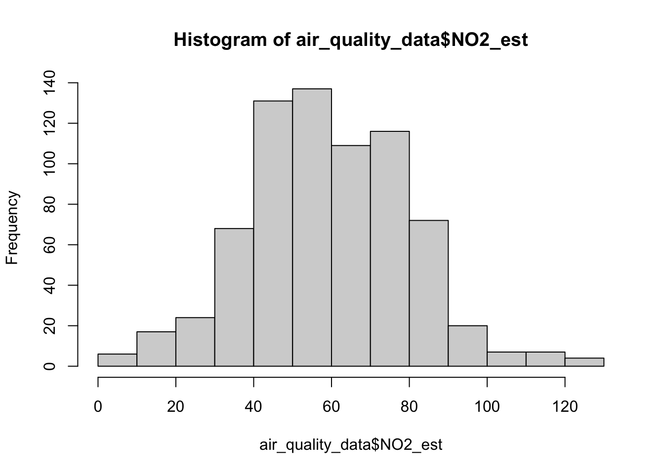
The above graph is not publication-worthy. It is missing key details such as the title and label for the x-axis. Let’s apply some cosmetics such as a main title and label for the x-axis
hist(air_quality_data$NO2_est, breaks = classes, main = "Histogram for NO2 in Barcelona", xlab = "NO2 estimates (ppb)")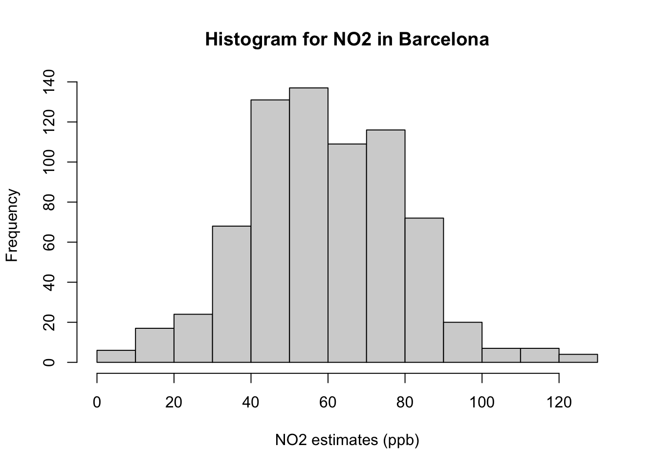
Interpretation of histogram: The above figure output describes the shape for ambient measures of NO\(_2\) in Barcelona which appears bell-shaped centered around 60ppb. Note that the frequency bars in this graph are essentially the same as the frequency values in the table.
Lastly, we then compute its cumulative frequency with cumsum() to support the interpretation. The coding needs a bit of hacking because we need to force a starting zero element for this graph to work.
cumfreq0 <- c(0, cumsum(frequency_results$Frequency))
plot(classes, cumfreq0, main="Cumulative Frequency for N02 in Barcelona", xlab="NO2 estimates (ppb)", ylab="Cumulative Frequencies")
lines(classes, cumfreq0) 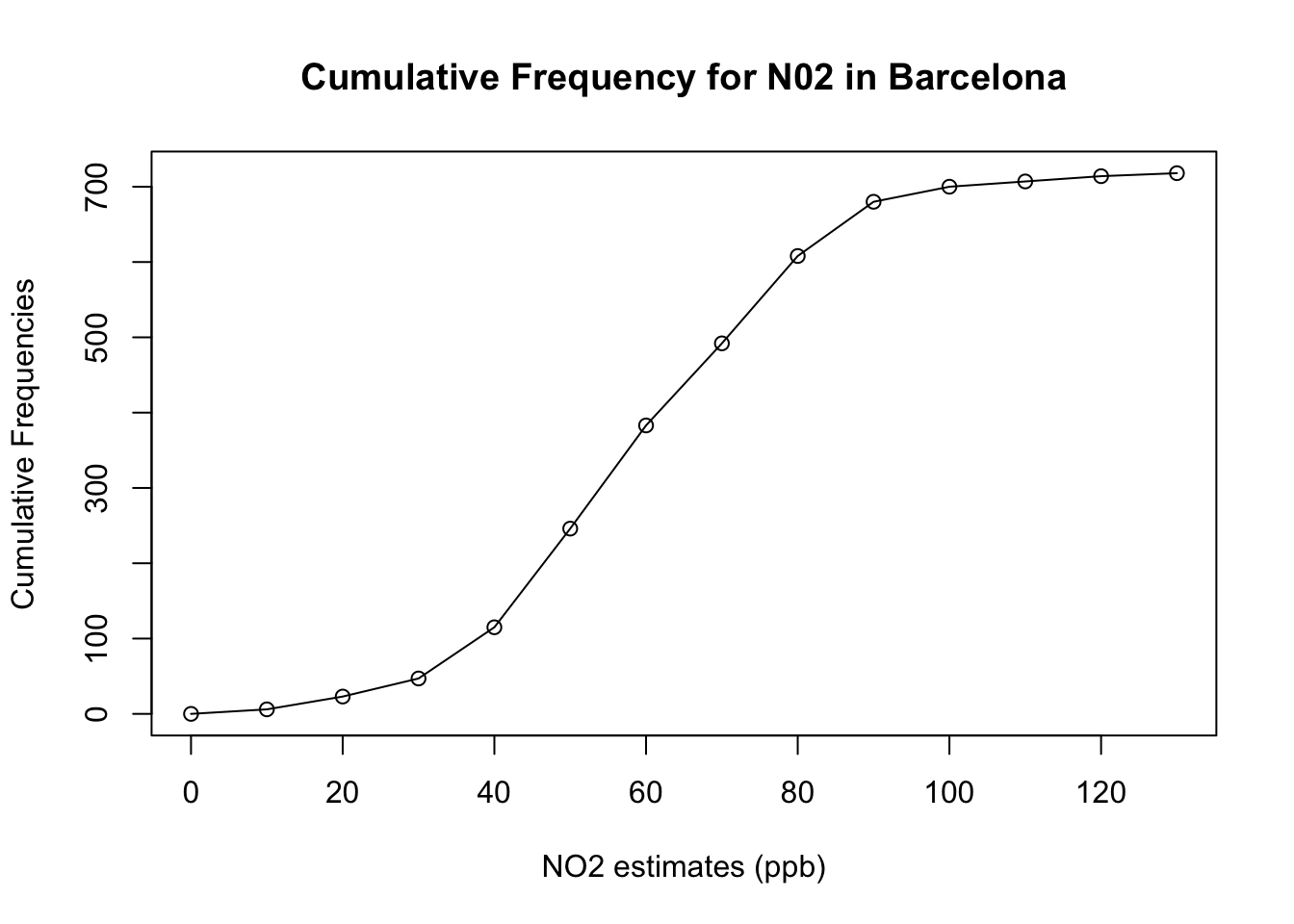
Descriptive and central tendency measures
We have used frequency distribution to describe the distribution about the data for air pollution in Barcelona. The description is at face-value though. Central tendency measures contains a list of summary measurements that allows the user to summarize the data to some central measure and to gauge the spread of the data (i.e., errors/departures from central measure). It is best for continuous variables, we can hence compute the following summary measurements (watch video below see to definitions):
- Mean
- Median
- Variance and Standard deviation
- Minimum and Maximum values
- Upper and Lower Quartiles (or Interquartile ranges)
[Theory]: Central tendency measures (Length: 17:12 minutes)
Watch on YouTube LINK
[Theory]: Range values and interquartile ranges (Length: 18:32 minutes)
Watch on YouTube [LINK]
To compute the summary statistics rapidly – simply use the summary() function on the variable of interest (i.e., NO2_est from the original dataset).
##    Min. 1st Qu.  Median    Mean 3rd Qu.    Max.
##    2.00   46.00   59.00   59.69   74.00  130.00
As you can see using summary() automatically gives you almost all the summary estimates needed for interpretation. The NO\(_2\) air levels in Barcelona was 59.69ppb (with median 59.00pbb). The lowest and highest values are 2.0ppb and 130.0ppb, respectively (with 25th and 75th percentiles being 46.00ppb and 74.00pbb, respectively.) Finally, you can compute the standard deviation using the sd() function as follows for income:
## [1] 20.60876[Theory]: Variance & standard deviation (Length: 13:39 minutes)
Watch on YouTube [LINK]
The standard deviation is ± 20.61pbb – this is the error around the mean of NO\(_2\) i.e., estimated as 59.69ppb. To visualise the distribution of a continuous variable – your ‘go-to’ plot is a boxplot. You can use the function boxplot() to generate one. Type the following to churn it:
# Box plot
boxplot(air_quality_data$NO2_est, ylab = "NO2 estimates (ppb)", main="Box plot: Summary of Nitrogen Dioxide in Barcelona")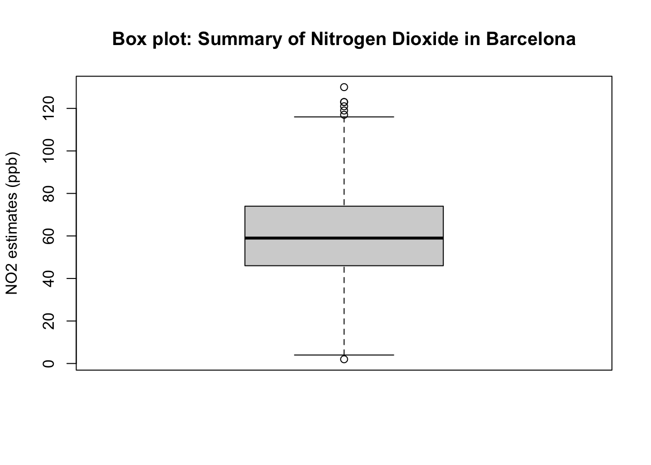
The above box plot is essential the visual representation of the summary results churned by the summary(). Here is the concise interpretation of the above results:
Interpretation: The overall mean air pollution levels for NO\(_2\) in Eixample (Barcelona) from 718 observation was 59.69ppb (with one SD of ± 20.63ppb). 25% (at the lower end i.e., lower quartile) of the distribution for air population levels for Nitrogen Dioxide are below 46.00ppb (which is considered to cause low health impact); while from 75% onwards (i.e., upper quartile) of the distribution has air pollution levels of N0\(_2\) which is above 74.00pbb (which is consider to considered to cause some moderate health impact). The overall range in the distribution is 128ppb where the lowest observed value is 2.0ppb (minimum) and the highest observed value is 130ppb (maximum)