Week 2 Examining data I
2.1 Introduction
Welcome to your second week of Introduction to Quantitative Research Methods. This week we will focus on examining data using measures of central tendency and measures of dispersion. These measures are collectively known as descriptive statistics. We will also talk about some basic data visualisation. Also, as by now, everyone should be up and running with RStudio Server, we will apply some of these descriptive measures onto some data. Alright, let’s get to it.
2.2 Measures of central tendency
Any research project involving quantitative data should start with an exploration and examination of the available data sets. This applies both to data that you have collected yourself and data that you have acquired in a different way, e.g., through downloading official UK Census and labour market statistics. The set of techniques that is used to examine your data in first instance is called descriptive statistics. Descriptive statistics are used to describe the basic features of your data set and provide simple summaries about your data. Together with simple visual analysis, they form the basis of virtually every quantitative data analysis.
2.2.1 Accessing RStudio Server, uploading and importing data
Make sure to download the data set for Week 2 from HERE if you have not already done so from the Welcome Page. The data sets are:
- For the tutorial practicals:
London historical population dataset.csv - For the seminar tasks and questions:
Ambulance and Assault Incidents data.csv
Let’s us first sign into RStudio Server:
- Log into the RStudio Server: https://rstudio.data-science.rc.ucl.ac.uk/. Log in with your usual UCL username and password.
- Create a new folder called
Week 2 - Upload the data
London historical population dataset.csvinto the folder ofWeek 2 - Set the directory to the folder location of
Week 2to where the CSV file was uploaded by clicking on theMore>>Set As Working Directory. - Finally, import the data into workspace using the
read.csv()function.
# Load data into RStudio. The spreadsheet is stored in the object called 'London.Pop'
London.Pop <- read.csv("London historical population dataset.csv")
If you struggle with the above steps, as well as setting up your working directory. Then here is a reminder, have a look at how we did this last week!
Use the head(), or View() functions to examine the structure of the London population data frame. The head() functions allows the users to see the first 5 rows of the data frame in the R-Console. The View() allows the user to see the entire spreadsheet in a data viewer.
2.2.2 Mean, Median and Mode
We are going to use the following functions: mean() and median(), to compute the mean and median value respectively - these two estimates are one of the three measures of central tendency.
We can apply these measures on our London.Pop data set. Let’s do this by focusing on London’s population in 2011. We going to keep the 1st, 2nd and 24th columns in the London.Pop data frame which corresponds to the columns called Area Code, Area Name and Person-2011, respectively.
Now we can calculate our measures of central tendency using R’s built-in functions for the median and the mean.
## [1] 254096## [1] 247695.2Question(s)
- How do you explain that the median is larger than the mean for this variable? [HINT: What is distorting the mean value such that its brought the value down?]
R does not have a standard in-built function to calculate the mode. As we still want to show the mode, we create a user function to calculate the mode of our data set. This function takes a numeric vector as input and gives the mode value as output.
Note
You do not have to worry about creating your own functions, so just copy and paste the code below to create the get_mode() function.
# create a function to calculate the mode
get_mode <- function(x) {

  # get unique values of the input vector
  uniqv <- unique(x)

  # select the values with the highest number of occurrences
  uniqv[which.max(tabulate(match(x, uniqv)))]
}
# calculate the mode of the 2011 population variable
get_mode(London.Pop2011$Persons.2011)
## [1] 7375Question(s)
- What is the level of measurement of our Persons.2011 variable? Nominal, ordinal, or interval/ratio?
- Even though we went through all the trouble to create our own function to calculate the mode, do you think it is a good choice to calculate the mode for this variable? Why? Why not?
Although R does most of the hard work for us, especially with the mean() and the median() function, it is a good idea to once go through the calculations of these two central tendency measures ourselves. Let’s calculate the mean step-by-step and then verify our results with the results of R’s mean() function.
# get the sum of all values
Persons.2011.Sum <- sum(London.Pop2011$Persons.2011)
# inspect the result
Persons.2011.Sum
## [1] 8173941# get the total number of observations
Persons.2011.Obs <- length(London.Pop2011$Persons.2011)
# inspect the result
Persons.2011.Obs## [1] 33# calculate the mean
Persons.2011.Mean <- Persons.2011.Sum / Persons.2011.Obs
# inspect the result
Persons.2011.Mean## [1] 247695.2# compare our result with R's built-in function
mean(London.Pop2011$Persons.2011) == Persons.2011.Mean## [1] TRUEGreat. Our own calculation of the mean is identical to R’s built-in function. Now let’s do the same for the median.
# get the total number of observations
Persons.2011.Obs <- length(London.Pop2011$Persons.2011)
# inspect the result
Persons.2011.Obs
## [1] 33# order our data from lowest to highest
Persons.2011.Ordered <- sort(London.Pop2011$Persons.2011, decreasing=FALSE)
# inspect the result
Persons.2011.Ordered## [1] 7375 158649 160060 182493 185911 186990 190146 199693 206125 219396
## [11] 220338 231997 237232 239056 246270 253957 254096 254557 254926 258249
## [21] 273936 275885 278970 288283 303086 306995 307984 309392 311215 312466
## [31] 338449 356386 363378# get the number of the observation that contains the median value
Persons.Median.Obs <- (Persons.2011.Obs + 1)/2
# inspect the result
Persons.Median.Obs## [1] 17# get the median
Persons.2011.Median <- Persons.2011.Ordered[Persons.Median.Obs]
# inspect the result
Persons.2011.Median## [1] 254096# compare our result with R's built-in function
median(London.Pop2011$Persons.2011) == Persons.2011.Median## [1] TRUE2.3 Simple plots
Before moving on to the second set of descriptive statistics, the measures of dispersion, this is a good moment to note that simple data visualisations are also an extremely powerful tool to explore your data. In fact, tools to create high quality plots have become one of R’s greatest assets. This is a relatively recent development since the software has traditionally been focused on the statistics rather than visualisation. The standard installation of R has base graphic functionality built in to produce very simple plots. For example we can plot the relationship between the London population in 1811 and 1911.
Note
Next week we will be diving deeper into data visualisation and making plots and graphs in R, but for now it is a good idea to already take a sneak peek at how to create some basic plots.
# make a quick plot of two variables of the London population data set
plot(London.Pop$Persons.1811,London.Pop$Persons.1911)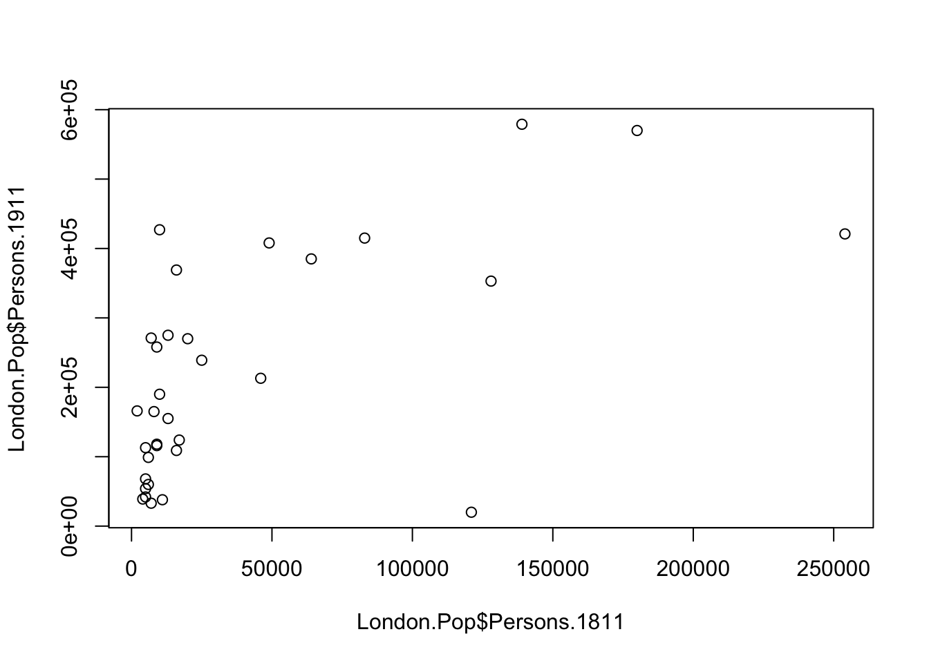
Experimenting with plot()
- What happens if you change the order of the variables you put in the
plot()function? Why? - Instead of using the
$to select the columns of our data set, how else can we get the same results?
The result of calling the plot() function, is a very simple scatter graph. The plot() function offers a huge number of options for customisation. You can see them using the ?plot help pages and also the ?par help pages (par in this case is short for parameters). There are some examples below (note how the parameters come after specifying the x and y columns).
# add a title, change point colour, change point size
plot(London.Pop$Persons.1811, London.Pop$Persons.1911, main='Quick Plot in R', col='blue', cex=2)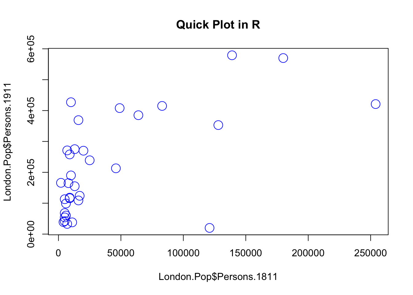
# add a title, change point colour, change point symbol
plot(London.Pop$Persons.1811, London.Pop$Persons.1911, main="Another Quick Plot in R", col='magenta', pch=22)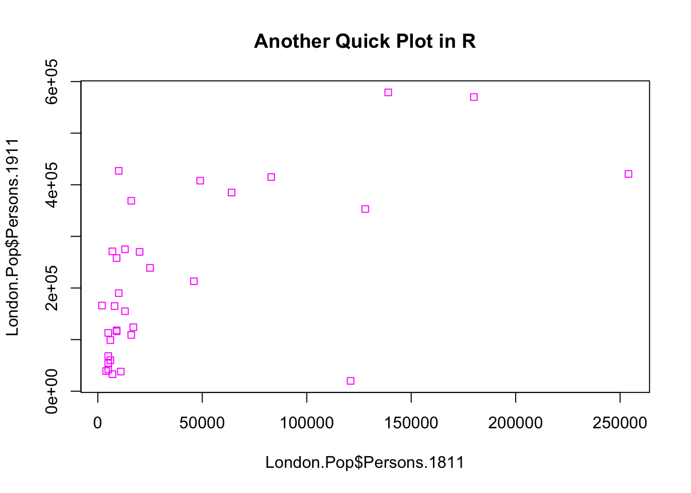
Also, you can apply titles to the axes using the xlab ="" and ylab="" argument after the main="" in the plot().
# add a axis titles, rotate number labels
plot(London.Pop$Persons.1811, London.Pop$Persons.1911, main="Another Quick Plot in R", xlab = "Population in 1811", ylab = "Population in 1911", col='magenta', pch=22)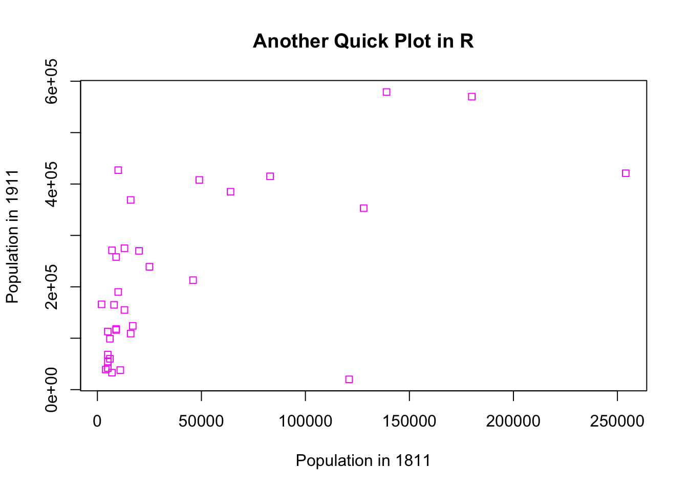
You can prevent R from printing the scientific notation (e.g., 2e+05, 4e+05 etc.,) on the y-axis in the graphical output. You can turn it off by typing the following code before running the plot() function
# turn-off horrible scientific notation
options(scipen = 999)
# add a axis titles, rotate number labels
plot(London.Pop$Persons.1811, London.Pop$Persons.1911, main="Another Quick Plot in R", xlab = "Population in 1811", ylab = "Population in 1911", col='magenta', pch=22)
Note
For more information on the plot parameters (some have obscure names) have a look here: http://www.statmethods.net/advgraphs/parameters.html
2.4 Measures of dispersion
When exploring your data, measures of central tendency alone are not enough as they only tell you what a ‘typical’ value looks like but they do not tell you anything about all other values. Therefore we also need to look at some measures of dispersion. Measures of dispersion describe the spread of data around a central value (e.g. the mean, the median, or the mode). The most commonly used measure of dispersion is the standard deviation. The standard deviation is a measure to summarise the spread of your data around the mean. The short video below will introduce you to the standard deviation as well as to three other measures of dispersion: the range, the interquartile range, and the variance.
For the rest of this tutorial we will change our data set to one containing the number of assault incidents that ambulances have been called to in London between 2009 and 2011. You will need to download a prepared version of this file called: Ambulance and Assault Incidents data.csv and upload it to your working directory. It is in the same data format (csv) as our London population file so we use the read.csv() command again.
# Load data into RStudio. The spreadsheet is stored in the object called 'London.Ambulance'
London.Ambulance <- read.csv('Ambulance and Assault Incidents data.csv')## BorCode WardName WardCode WardType Assault_09_11
## 1 00AA Aldersgate 00AAFA Prospering Metropolitan 10
## 2 00AA Aldgate 00AAFB Prospering Metropolitan 0
## 3 00AA Bassishaw 00AAFC Prospering Metropolitan 0
## 4 00AA Billingsgate 00AAFD Prospering Metropolitan 0
## 5 00AA Bishopsgate 00AAFE Prospering Metropolitan 188
## 6 00AA Bread Street 00AAFF Prospering Metropolitan 0## [1] 649 5You will notice that the data table has 5 columns and 649 rows. The column headings are abbreviations of the following:
| Column heading | Full name | Description |
|---|---|---|
| BorCode | Borough Code | London has 32 Boroughs (such as Camden, Islington, Westminster, etc.) plus the City of London at the centre. These codes are used as a quick way of referring to them from official data sources. |
| WardName | Ward Name | Boroughs can be broken into much smaller areas known as Wards. These are electoral districts and have existed in London for centuries. |
| WardCode | Ward Code | A statistical code for the wards above. |
| WardType | Ward Type | A classification that groups wards based on similar characteristics. |
| Assault_09_11 | Assault Incidents | The number of assault incidents requiring an ambulance between 2009 and 2011 for each ward in London. |
Let’s start by calculating two measures of central tendency by using the median() and mean() functions.
## [1] 146## [1] 173.4669Questions
- How do you explain that the mean is larger than the median for this variable?
Great. Let’s now calculate some measures of dispersion for our data: the range, the interquartile range, and the standard deviation. The calculation of the range is very straightforward as we only need to subtract the the minimum value from the the maximum value. We can find these values by using the built-in min() and max() functions.
## [1] 0## [1] 1582## [1] 1582## [1] 1582Questions
- What does this range mean?
The interquartile range requires a little bit more work to be done as we now need to work out the values of the 25th and 75th percentile.
Note
A percentile is a score at or below which a given percentage of your data points fall. For example, the 50th percentile (also known as the median!) is the score at or below which 50% of the scores in the distribution may be found.
# get the total number of observations
London.Ambulance.Obs <- length(London.Ambulance$Assault_09_11)
# inspect the result
London.Ambulance.Obs
## [1] 649# order our data from lowest to highest
London.Ambulance.Ordered <- sort(London.Ambulance$Assault_09_11, decreasing=FALSE)
# inspect the result
London.Ambulance.Ordered## [1] 0 0 0 0 0 0 0 0 0 0 0 0 0 0 0
## [16] 0 10 18 19 21 22 25 28 28 28 29 30 34 36 36
## [31] 38 40 41 41 42 42 42 43 43 44 44 45 46 46 47
## [46] 47 48 48 48 49 49 49 49 49 50 50 50 51 51 51
## [61] 51 51 51 52 53 53 54 54 54 55 55 55 56 56 56
## [76] 56 57 57 57 57 57 58 59 59 60 61 62 63 63 64
## [91] 64 64 64 64 64 64 65 65 65 66 66 66 67 67 67
## [106] 68 69 69 69 69 70 70 71 71 71 71 72 73 74 74
## [121] 74 74 75 75 75 76 76 76 76 76 76 76 77 77 77
## [136] 77 77 77 78 78 78 79 79 79 80 80 80 80 81 81
## [151] 82 82 82 83 83 84 85 85 85 86 86 86 86 87 87
## [166] 87 87 87 88 88 88 89 89 89 89 89 91 91 93 93
## [181] 94 94 96 97 97 97 98 98 98 99 99 100 100 101 102
## [196] 102 102 102 102 103 104 105 105 105 105 105 106 107 107 107
## [211] 108 108 108 108 109 109 109 109 110 110 110 110 111 111 112
## [226] 112 113 113 113 113 114 114 114 114 114 114 115 115 116 116
## [241] 117 117 117 117 118 118 119 119 119 119 119 120 120 120 121
## [256] 121 122 122 122 123 124 124 125 125 125 125 125 125 126 127
## [271] 127 127 127 128 128 128 129 129 130 130 130 131 131 131 132
## [286] 132 132 132 132 133 133 134 135 135 135 137 137 138 138 138
## [301] 138 138 139 139 140 141 142 142 142 142 143 143 143 143 144
## [316] 144 144 144 145 145 145 146 146 146 146 146 146 148 148 148
## [331] 149 150 150 150 151 151 152 152 152 153 153 153 153 154 155
## [346] 155 155 156 156 157 157 157 157 158 158 158 158 160 161 161
## [361] 161 161 162 162 163 163 164 164 165 165 166 167 169 169 170
## [376] 170 170 171 171 172 172 175 175 175 176 178 178 180 181 181
## [391] 181 182 182 182 183 183 184 184 184 185 185 185 186 188 190
## [406] 190 190 191 192 192 193 193 193 194 194 194 194 194 194 195
## [421] 195 195 195 196 196 196 197 198 198 199 200 200 201 201 201
## [436] 202 203 204 205 206 206 208 208 208 208 208 209 209 209 210
## [451] 210 210 210 212 212 212 213 213 213 213 214 215 215 216 217
## [466] 220 220 221 221 222 222 222 224 225 226 226 227 229 229 230
## [481] 230 231 232 232 232 232 233 233 234 234 235 235 236 237 237
## [496] 238 238 240 243 243 244 245 245 245 247 247 247 248 249 251
## [511] 251 251 251 252 252 253 253 253 254 255 257 257 258 258 258
## [526] 258 259 259 259 260 260 260 261 264 265 265 266 267 267 268
## [541] 270 271 272 272 273 273 274 274 274 278 278 278 279 281 283
## [556] 283 283 284 285 287 288 290 291 292 292 293 293 294 295 296
## [571] 296 297 300 300 302 303 304 305 306 306 313 314 315 315 315
## [586] 315 318 319 321 324 325 326 326 328 329 331 334 334 339 339
## [601] 339 341 342 347 350 352 352 355 358 359 361 363 365 365 366
## [616] 369 371 371 374 376 378 383 405 407 409 420 429 429 435 437
## [631] 437 442 457 458 464 467 473 482 484 495 502 535 542 573 579
## [646] 602 765 1305 1582# get the number ('index value') of the observation that contains the 25th percentile
London.Ambulance.Q1 <- (London.Ambulance.Obs + 1)/4
# inspect the result
London.Ambulance.Q1## [1] 162.5# get the number ('index value') of the observation that contains the 75th percentile
London.Ambulance.Q3 <- 3*(London.Ambulance.Obs + 1)/4
# inspect the result
London.Ambulance.Q3## [1] 487.5## [1] 86## [1] 233## [1] 147As explained at the very end of this lecture video, we can also visually represent our range, median, and interquartile range using a box and whisker plot:
# make a quick boxplot of our assault incident variable
boxplot(London.Ambulance$Assault_09_11, horizontal=TRUE)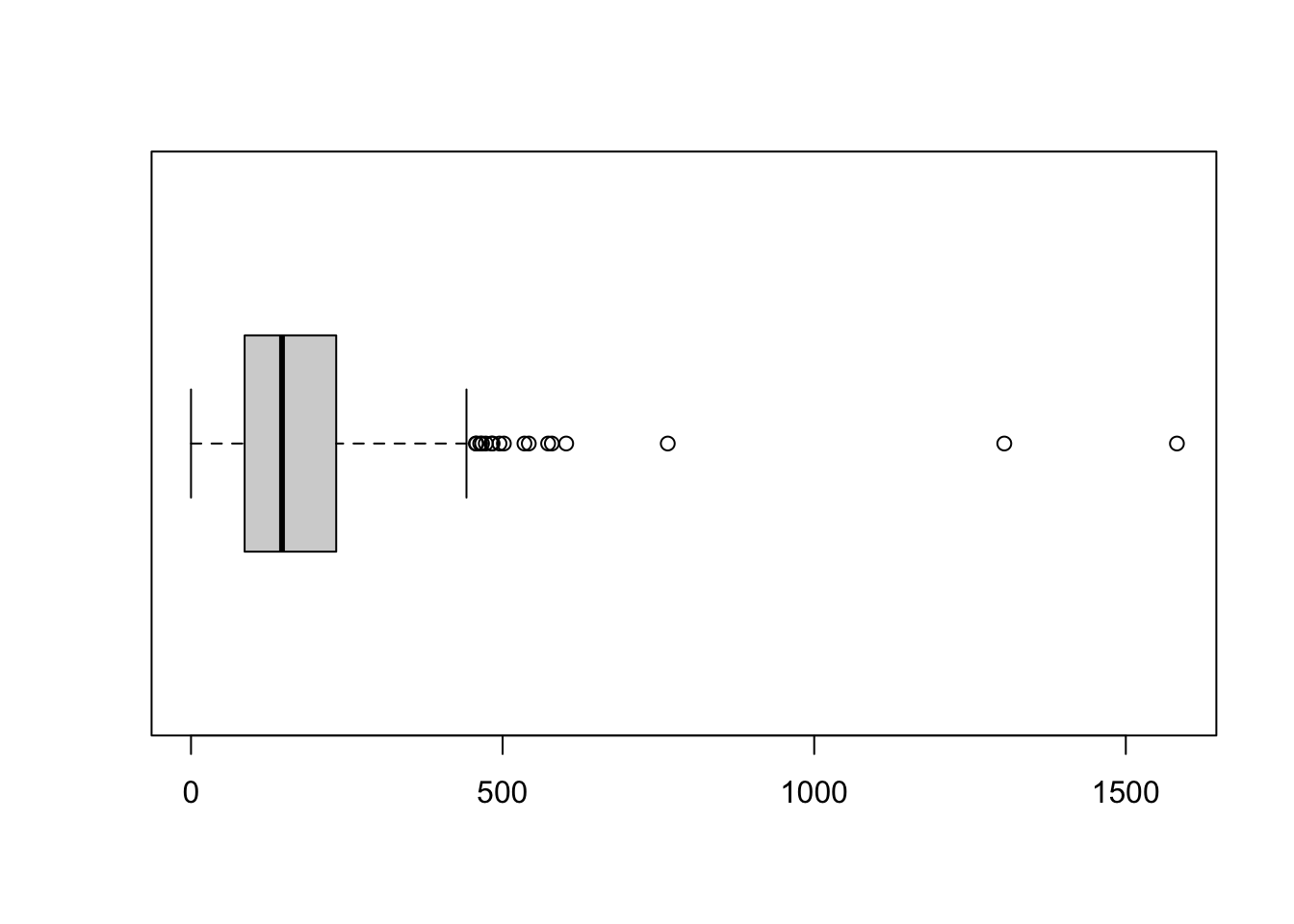
Questions
- There is a large difference between the range that we calculated and the interquartile range that we calculated. What does this mean?
- The 25th and 75th percentile in the example do not return integer but a fraction (i.e. 162.5 and 487.5). Why do we use 163 and 488 to extract our percentile values and not 162 and 487?
Now, let’s move to the standard deviation. Remember: this is one of the most important measures of dispersion and is widely used in all kinds of statistics. The calculation involves the following steps as extensively explained in this lecture video:
- Calculate the mean.
- Subtract the mean from each observation to get a residual.
- Square each residual.
- Sum all residuals.
- Divide by \(n-1\).
- Take the square root of the final number.
# calculate the mean
London.Ambulance.Mean <- mean(London.Ambulance$Assault_09_11)
# subtract the mean from each observation
London.Ambulance.Res <- London.Ambulance$Assault_09_11 - London.Ambulance.Mean
# square each residual
London.Ambulance.Res.Sq <- London.Ambulance.Res**2
# sum all squared residuals
London.Ambulance.Res.Sum <- sum(London.Ambulance.Res.Sq)
# divide the sum of all sqaured residuals by n - 1
London.Ambulance.Variance <- London.Ambulance.Res.Sum / (length(London.Ambulance$Assault_09_11) - 1)
# take the square root of the final number
London.Ambulance.Sd <- sqrt(London.Ambulance.Variance)
# standard deviation
London.Ambulance.Sd
## [1] 130.3482There we go. We got our standard deviation! You probably already saw this coming, but R does have some built-in functions to actually calculate these descriptive statistics for us: range(), IQR(), and sd() will do all the hard work for us!
## [1] 0 1582## [1] 147## [1] 130.3482Note
Please be aware that the IQR() function may give slighlty different results in some cases when compared to a manual calculation. This is because the forumula that the IQR() function uses is slightly different than the formula that we have used in our manual calculation. It is noted in the documentation of the IQR() function that: “Note that this function computes the quartiles using the quantile function rather than following Tukey’s recommendations, i.e., IQR(x) = quantile(x, 3/4) - quantile(x, 1/4).”
Questions
- What does it mean that we have a standard deviation of 130.3482?
- Given the context of the data, do you think this is a low or a high standard deviation?
To make things even easier, R also has a summary() function that calculates a number of these routine statistics simultaneously. After running the summary() function on our assault incident variable, you should see you get the minimum (Min.) and maximum (Max.) values of the assault_09_11 column; its first (1st Qu.) and third (3rd Qu.) quartiles that comprise the interquartile range; its the mean and the median. The built-in R summary() function does not calculate the standard deviation. There are functions in other libraries that calculate more detailed descriptive statistics,
# calculate the most common descriptive statistics for the assault incident variable
summary(London.Ambulance$Assault_09_11)
## Min. 1st Qu. Median Mean 3rd Qu. Max.
## 0.0 86.0 146.0 173.5 233.0 1582.02.5 Seminar task & questions
Seminar Task: Use the seminar, you will be continuing with the data set Ambulance and Assault Incidents data.csv. Still work with the data frame object named as London.Ambulance.
- Create a new object / data set that only contains data for ward type Suburbs and Small Towns. Hint: Try to subset the data by filtering it based on
WardType. - Calculate the mode, median, mean, range, interquartile range, and standard deviation for the Assault_09_11 variable for Suburbs and Small Towns
- Produce a
boxplot()that provides a visual description of it’s distribution
Seminar questions
Compare the results of the descriptive statistics you have calculated for your Suburbs and Small Towns object with the results of the descriptive statistics you have calculated for you Prospering Metropolitan object / data set.
- What do these differences tell us about the levels of violent assaults within these separate environments?
- Create a dual boxplot to show a visual representation of this comparison.
Important Note: The solution codes will be released next week on Monday. Oh yeah - before you leave, do save your R script by pressing the Save button in the script window. You survived - that is it for this week!