Week 1 Understanding Data
1.1 Lecture video (Length: 02:00:01)
Important Note: This resource contains the recorded lectures, which are provided for your convenience as a supplementary resource if you have already attended the lectures. Please note that watching the lecture recordings alone will not be sufficient to fully grasp the material or adequately prepare for the final assessment.
POLS0008 is a practical module that requires consistent weekly engagement in both lectures and seminars. Please be aware that seminars are not recorded. Additionally, while every effort has been made to ensure clarity, module tutors cannot guarantee top-quality audio or video footage.
1.2 Introduction
Welcome to week 1’s practicals for Introduction to Quantitative Research Methods. This week we will focus on understanding data. The goal for this week’s session is to get you started with using RStudio and getting you to become familiar with its environment. Today’s session aims to introduce you to the basic programming etiquette as well as building your confidence in using RStudio. At the end of this session, you should be able to perform the following:
- Accessing RStudio Server from a UCL Workstation or remotely
- Use the R-Console as a basic calculator
- Loading in data from a CSV & sub-setting it into smaller chunks
- Handle discrete and categorical data
- Basic graphical visualisation in RStudio
Make sure to download the data set for Week 1 from HERE if you have not already done so from the Welcome Page, as we will use them later on in Sections 1.7. and 1.9.. The data sets are:
- For the tutorial practicals (Section 1.7.):
Primary Schools in Ealing.csv - For the seminar tasks and questions (Section 1.9.):
All Schools in London.csv
At the end of this tutorial, you will be asked to complete the tasks and questions in Section 1.9. Do try to complete this before Thursday’s seminar session. The solutions to Section 1.9 will be released with the week’s new lecture notes and other content.
1.3 Instructions for accessing RStudio Server
To begin, we provide a step-by-step guide to accessing RStudio Server on your personal computer. Please note that you must be connected to UCL’s Network.
OPTION A - Connecting to RStudio Server from laptop/PC when connected directly to UCL’s EDUROAM:
- Make sure you are already connected to UCL’s EDUROAM wifi if you are on campus.
- Open any web browser (i.e., Internet Explorer, Google Chrome, Safari etc.) and navigate to the browser and type the following link: https://rstudio.data-science.rc.ucl.ac.uk/.
- Log in with your usual UCL username and password. You should see the RStudio interface appear.
OPTION B - Connecting from a personal device:
Alternatively, if you are working on your laptop/PC off-campus, you can still access RStudio Server. However, you will need to work remotely via Desktop @ UCL Anywhere from your personal device and connect through there.
Video explanation (Length: 12:04 minutes)
Here are the following steps:
- Initiate UCL Remote Desktop @ Anywhere, click on this LINK
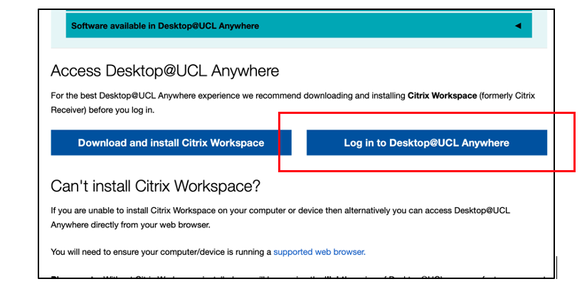
- Next, click on the ‘Log in to Desktop @ UCL Anywhere’ blue button to log in, and then select “Use Light Version” or “Web Browser”.

- A page will appear asking you to enter your UCL username and password, enter these pieces of information, and click “Log On”.
![]()
Click on the icon “Desktop @ UCL Anywhere” to initiate the remote access on to a UCL workstation
You are now in the network remotely. To open RStudio Server simply open any web browser (i.e., Internet Explorer or Google Chrome) within the remote environment and go to this link: https://rstudio.data-science.rc.ucl.ac.uk/. Log in with your usual UCL username and password and you should see the RStudio interface appear.
1.4 The environment in RStudio
When opening RStudio for the first time, you are greeted with its interface. The window is split into three panels: 1.) R-Console, 2.) Environments and 3.) Files, help & Output.
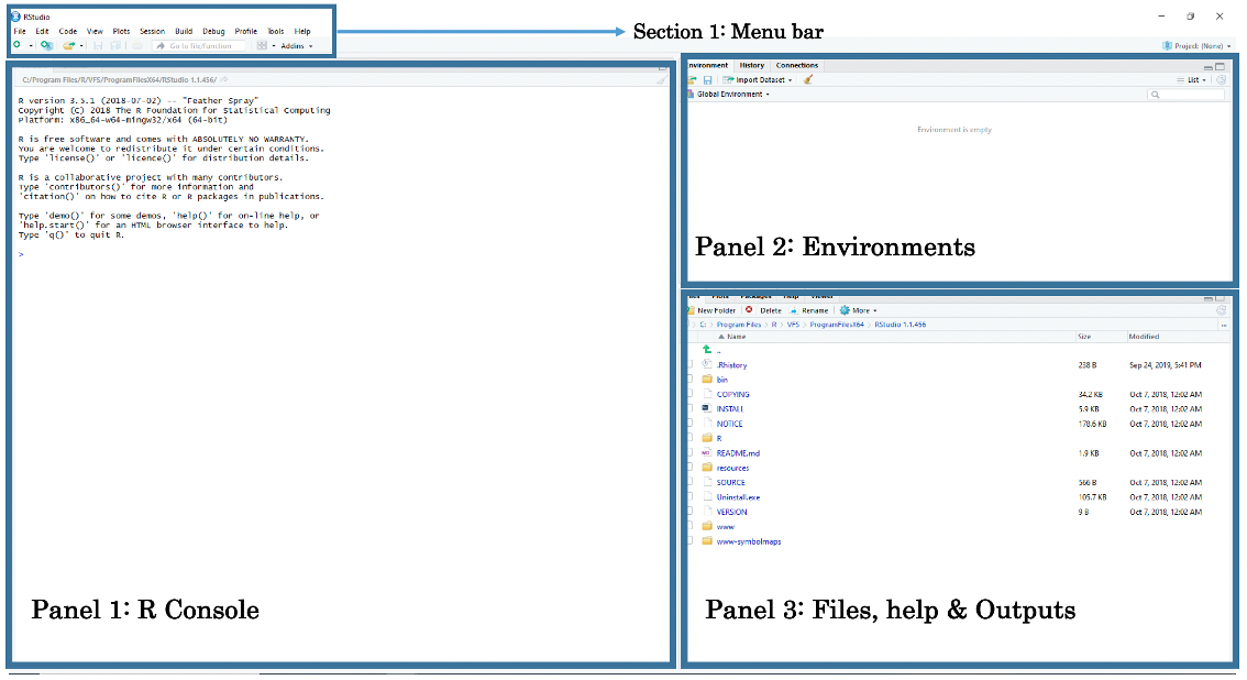
Panel 1: The R-Console lets the user type in R-codes to execute rapid commands and use it as basic calculator.
Panel 2: The Environments lets the user see which data sets, objects and other files are currently stored in RStudio’s memory
Panel 3: Under the File tab, it lets the user access other folders stored in the computer to open datasets. Under the Help tab, it also allows the user to view the help menu for codes and commands. Finally, under the Plots tab, the user can perusal his/her generated plots (e.g., histogram, scatter plots, maps etc.).
The above section is the Menu Bar. You can access other functions for saving, editing, and opening a new Script File for writing codes. When you open a Script File, it reveals a fourth panel above the R-Console.
You can open a Script File by simply going to the Menu Bar and clicking on “New File” >> “R Script”. This should open a new Script File titled ‘Untitled 1’.
In all practical tutorials, you will be encouraged to use an R Script for collating and saving the codes written for these analyses. We will start writing codes in a script from section 1.7 on wards. For now, let us start with the absolute basics, we begin with interacting with the R-Console as a basic calculator and typing in some simple code.
1.5 Using the R-Console as a calculator
The R console window (i.e., Panel 1) is the place where RStudio is waiting for you to tell it what to do. It will show the code you have commanded RStudio to execute, and it will also show the results from that command. You can type the commands directly into the window for execution of as well.
Video explanation (Length: 13:35 minutes)
Let us start by using the console window as a basic calculator for typing in addition (+), subtraction (-), multiplication (*), division (/) and performing other complex sums. Click inside the R Console window and type 19+8, and press enter button to get your answer.
Perform the following sums by typing them inside the R Console window:
## [1] 27## [1] -69## [1] 360## [1] 9## [1] 1011.154Important Note: The text that follows after the hash tag # in the above code chunk is a comment and NOT actual code. I have put those comments there to tell you what the code below it (i.e., without hash tag # in front of it) what its doing.
Aside from basic arithmetic operations, we can use some basic mathematical functions such as the exponential and natural logarithms:
exp()is the exponential functionlog()is the logarithmic function^this symbol allows the user to raise a number to a power
Do not worry at all about these function as you will use them later in the weeks to come for transforming variables. For now, perform the following by typing them inside the R-Console window:
## [1] 148.4132## [1] 1.098612## [1] 2561.6 Creating basic objects and assigning values to them
Now that we are a bit familiar with using the console as a calculator. Let us build on this and learn one of the most important codes in RStudio which is Assignment Operator.
Video explanation (Length: 20:29 minutes)
This arrow symbol <- is called the Assignment Operator. It is typed by pressing the less than symbol < followed by the hyphen symbol -. It allows the user to assign values to an object.
Objects are defined as stored quantities in RStudio’s environment. These objects can be assigned anything from a numeric value to a string character. For instance, suppose we want to create a numeric object called x and assign it with a value of 3. We do this by typing x <- 3. Another example, suppose we want to create a string object called y and we assign it with some text "Hello!". We do this typing y <- "Hello!".
Let us create the objects a, b, c, and d and assign them with numeric values. Perform the following by typing them inside the R Console window:
# Create an object called 'a' and assign the value 17 to it
a <- 17

# Type the object 'a' in console as a command to return value 17
a
## [1] 17# Create an object called 'b' and assign the value 10 to it
b <- 10
# Type the object 'b' in console as a command to return value 10
b## [1] 10# Create an object called 'c' and assign the value 9 to it
c <- 9
# Type the object 'c' in console as a command to return value 9
c## [1] 9# Create an object called 'd' and assign the value 8 to it
d <- 8
# Type the object 'd' in console as a command to return value 8
d## [1] 8Notice how the objects a, b, c and d and its value are stored in RStudio’s environment panel. We can perform the following arithmetic operations with these object values:
## [1] 8.8## [1] 25Let us create more objects but this time we will assign character string(s) to them. Please note that when typing a string of characters as data in RStudio, you will need to cover them with quotation marks “…”. For example, suppose we want to create a string object called y and assign it with some text "Hello!". We do this by typing y <- "Hello!".
Try these examples of assigning the following character text to an object.
# Create an object called 'e' and assign the character string "RStudio"
e <- "RStudio"

# Type the object 'e' in the console as a command to return "RStudio"
e
## [1] "RStudio"# Create an object called 'f', assign character string "Hello world"
f <- "Hello world"
# Type the object 'f' in the console as a command to return "Hello world"
f## [1] "Hello world"# Create an object called 'g' and assign "Blade Runner is amazing"
g <- "Blade Runner is amazing"
# Type the object 'g' in the console to return the result
g## [1] "Blade Runner is amazing"We are now familiar with using the console and assigning (numeric and string) values to objects. The parts covered in from section 1.3 and 1.4 are the initial building blocks for coding & creating data sets.
Let us progress to section 1.5. From this point onwards, we will learn the basics of managing data and etiquettes, which includes creating data frames, as well as importing CSVs & saving R-objects as a CSV file, and setting up a work directory in RStudio server.
1.7 Data entry in RStudio
As you have already seen, RStudio is an object-oriented software package and so entering data is slightly different for the usual way when inputting information into a spreadsheet (e.g., Microsoft Excel etc.,). Here, you will need to enter the information as Vector objects before combining them into a Data Frame object.
Consider this incredibly Wishie Washy example of some data containing additional health information of 10 people. It contains the variable (or column) names 'id', 'name', 'height', 'weight' and 'gender'.
| id | name | height | weight | gender |
|---|---|---|---|---|
| 1 | Sam | 1.65 | 64.2 | M |
| 2 | Kofi | 1.77 | 80.3 | M |
| 3 | Kate | 1.70 | 58.7 | F |
| 4 | Cindy | 1.68 | 75.0 | F |
| 5 | Patel | 1.80 | 69.6 | M |
| 6 | James | 1.60 | 49.3 | M |
| 7 | Tatiana | 1.66 | 52.7 | F |
| 8 | Roberto | 1.71 | 40.0 | M |
| 9 | Rubio | 1.63 | 55.6 | M |
| 10 | Fatima | 1.73 | 62.5 | F |
In RStudio, data is entered as a sequence of elements and listed inside an object called a Vector. For instance, if we have three age values of 12, 57 and 26 years, and we want to enter this in RStudio, we need to use the function c() and combine these three elements into a Vector object.
Hence, the code will be c(12, 57, 26). We can assign this to something by typing this code age <- c(12, 57, 26). Any time you type age into RStudio console. It will return these three values unless you chose to overwrite it with different information.
Let us look at this more closely with the id variable from the above data. Each person has an ID number from 1 to 10. We are going to list the numbers 1, 2, 3, 4, 5, 6, 7, 8, 9 and 10 as a sequence of elements into a vector using c() and then assign it to as a vector object calling it id.
# Create 'id' vector object
id <- c(1, 2, 3, 4, 5, 6, 7, 8, 9, 10)

# Type the vector object 'id' in console to return output
id
## [1] 1 2 3 4 5 6 7 8 9 10Now, let us enter the same remaining columns for 'name', 'height', 'weight' and 'gender' like we did for ‘id’:
# Create 'name' vector object
name <- c("Sam", "Kofi", "Kate", "Cindy", "Patel", "Harry", "Kimba", "Roberto", "Rubio", "Fatima")

# Create 'height' (in meters) vector object
height <- c(1.65, 1.77, 1.70, 1.68, 1.80, 1.60, 1.66, 1.71, 1.63, 1.73)

# Create 'weight' (in kg) vector object
weight <- c(64.2, 80.3, 58.7, 75.0, 69.6, 49.3, 52.7, 40.0, 55.6, 62.5)

# Create 'gender' vector object
gender <- c("M", "M", "F", "F", "M", "M", "F", "M", "M", "F")
Now, that we have the vector objects ready. We can bring them together to create a proper data set. This new object is called a Data Frame. We need to list the vectors inside the data.frame() function.
# Create a dataset (data frame)
dataset <- data.frame(id, name, height, weight, gender)

# Type the data frame object 'dataset' in console to see output
dataset
## id name height weight gender
## 1 1 Sam 1.65 64.2 M
## 2 2 Kofi 1.77 80.3 M
## 3 3 Kate 1.70 58.7 F
## 4 4 Cindy 1.68 75.0 F
## 5 5 Patel 1.80 69.6 M
## 6 6 Harry 1.60 49.3 M
## 7 7 Kimba 1.66 52.7 F
## 8 8 Roberto 1.71 40.0 M
## 9 9 Rubio 1.63 55.6 M
## 10 10 Fatima 1.73 62.5 FImportant Note: The column ‘id’ is numeric variable with integers. The second column ‘name’ is a text variable with strings. The third & fourth columns ‘height’ and ‘weight’ are examples of a numeric variables with real numbers – both variables are continuous. The variable ‘gender’ is text variable with strings – however, this type of variable is classed as a categorical variable as individuals were categorised as either ‘M’ and ‘F’.
1.8 Uploading data to RStudio Server and importing data into the environment
We are going to import the downloaded data for Week 1 into RStudio. It contains information pertained to 58 primary schools in Ealing. We can open spreadsheets, particularly, CSV files in an organised way by uploading the file in the RStudio Server and then opening it using the read.csv() function.
Video explanation (Length: 12:16 minutes)
We can do this in four steps:
Step 1. Keep the space in your personal directory /nfs/cfs/home2/XXXX/ucl_username tidy by creating new folder and naming it Week 1 simply by clicking the New Folder button in the bottom-right panel.
Step 2. Next, click on the Week 1 folder to enter it, and then click on the Upload button and select the downloaded CSV file Primary Schools in Ealing.csv to be uploaded into the RStudio Server.
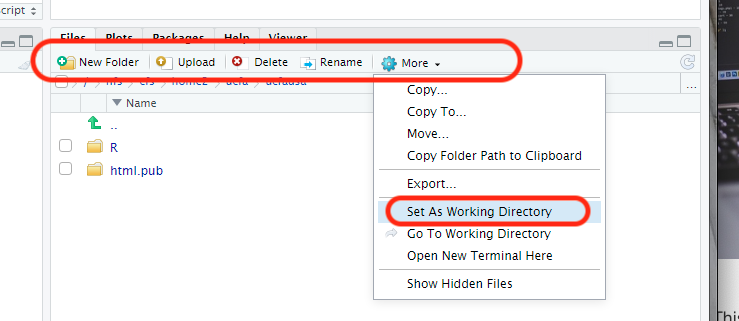
Step 3. We must set the directory to the folder location in the server to where the CSV file was uploaded by clicking on the More >> Set As Working Directory.
Step 4. Finally, we can import the data using the read.csv() function. The code syntax in the script should read as follows:
# Load data into RStudio. The spreadsheet is stored in the object called 'SchoolData'
SchoolData <- read.csv("Primary Schools in Ealing.csv")
The loaded dataset contains the following variables:
SchoolName: Name of school in Ealing (string)Type: School classified as a ‘Primary’ school (string)AgeGroup: Categorised as three age groups i.e.,3-11,4-11,7-11(categorical)NumberBoys: Total number of boys in a primary school (Discrete/counts)NumberGirls: Total number of girls in a primary school (Discrete/counts)TotalStudents: Total number of students in a primary school (Discrete/counts)OfstedGrade: Overall school performance1= excellent,2= good,3= requires improvement,4= inadequate (categorical)
We have learned a lot of basic things in RStudio, the stuff shown in this section in particular will be used quite a lot in future tutorials - so do get use to keep your space clean with new folders, and use uploading and importing data. Let us progress to the final section and learn some basics of working with imported data in R.
1.9 Working with data in RStudio
1.9.1 Useful functions
One can examine the structure of the imported data with the following basic functions.
str(): tells the user which columns in the data frame are character or numeric variableshead(): allows the user to see the first top 10 rows of the data frametail(): allows the user to see the last bottom 10 rows of the data framencol(): tells the user the total number of columns present in the data framenrow(): tells the user the total number of observations (or rows) present in the data framenames(): returns the list column names present in the data frame
## 'data.frame':    58 obs. of  6 variables:
##  $ SchoolName   : chr  "Berrymede Junior School" "East Acton Primary School" "Oldfield Primary School" "North Ealing Primary School" ...
##  $ Type         : chr  "Primary" "Primary" "Primary" "Primary" ...
##  $ NumberBoys   : int  180 160 225 340 265 230 155 285 185 150 ...
##  $ NumberGirls  : int  200 165 240 355 205 205 180 290 190 125 ...
##  $ TotalStudents: int  377 329 465 697 471 435 335 573 373 273 ...
## $ OfstedGrade : int 2 2 2 2 2 2 2 3 2 2 ...## [1] 58## [1] "SchoolName" "Type" "NumberBoys" "NumberGirls"
## [5] "TotalStudents" "OfstedGrade"You can examine specific variables from this data frame, for instance, we can get observation with the primary school that has the minimum and maximum number of students using the min() and max() function, respectively. We can also compute the total number primary students in Ealing using the sum().
We can compute these values using the $ symbol to select the column of interest, which is TotalStudents. Specify the name of the data frame (i.e., SchoolData) and then select the column of interest after the $
## [1] 891## [1] 239## [1] 294731.9.2 Basic subsetting and manipulation of data
One can subset or restrict the data frame by specifying which row(s) and column(s) to keep or discard using this square bracket notation dataframe[Row, Column].
For example:
## [1] "Berrymede Junior School"## [1] "Berrymede Junior School" "East Acton Primary School"
## [3] "Oldfield Primary School" "North Ealing Primary School"
## [5] "St John's Primary School"## SchoolName TotalStudents OfstedGrade
## 1 Berrymede Junior School 377 2
## 2 East Acton Primary School 329 2
## 3 Oldfield Primary School 465 2
## 4 North Ealing Primary School 697 2
## 5 St John's Primary School 471 2Another trick one can do is use other columns or variables within a data frame to create another variable. This technique is essentially important when cleaning and managing data.
From the data, we can derive proportion (%) of students who are boys for each school using $. Here, we can create a new column called PercentBoys as follows:
1.9.3 Basic visualisation
The school data only contains variables that are in counts or categories. Hence, we can only use visualisations such as pie charts or bar charts for such types of data (of course, in week 2, we’ll explore ways for visualising continuous data).
The OfstedGrade variable has classified schools according to the overall performance from 1 (outstanding) to 4 (poor). We can visual the frequency of schools by performance grade in a bar chart using barchart() function:
# tabulate the frequency of schools based on the OfstedGrade using table()
counts <- table(SchoolData$OfstedGrade)
counts
##
## 1 2 3 4
## 6 47 4 1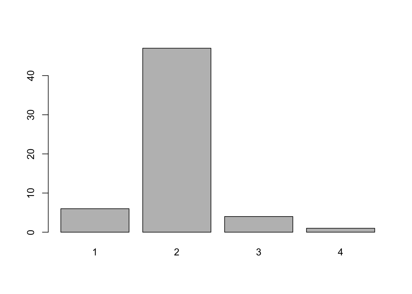
#Fully labelled Bar Plot
barplot(counts, main="School Distribution based on OFSTED performance", xlab ="OFSTED grades", ylab="Number of Schools")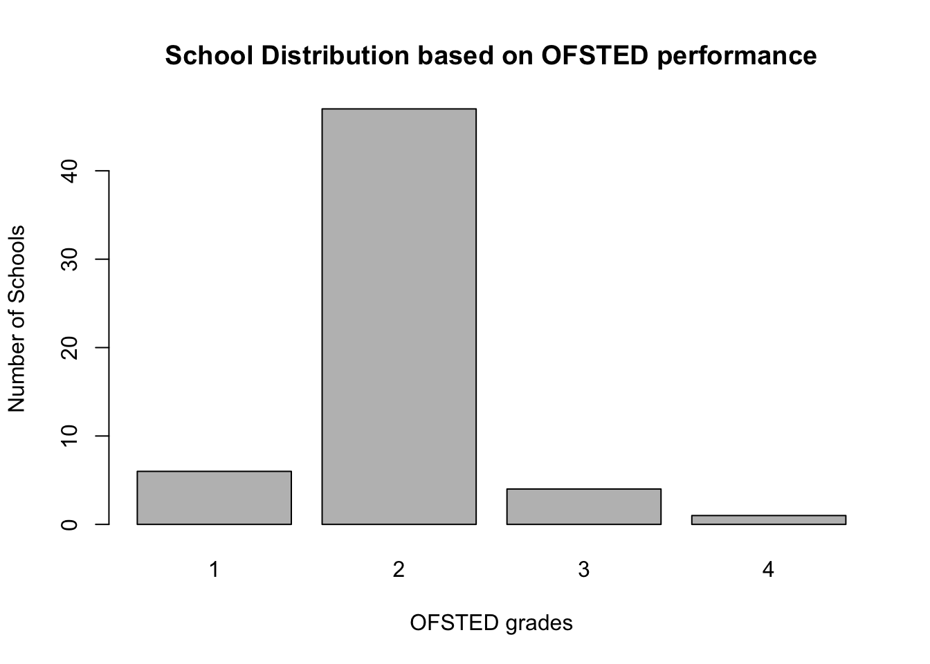
We can represent the above data again as a piechart reporting percentages instead using the pie()
# tabulate the frequency of schools based on the OfstedGrade using table()
counts <- table(SchoolData$OfstedGrade)
counts
##
## 1 2 3 4
## 6 47 4 1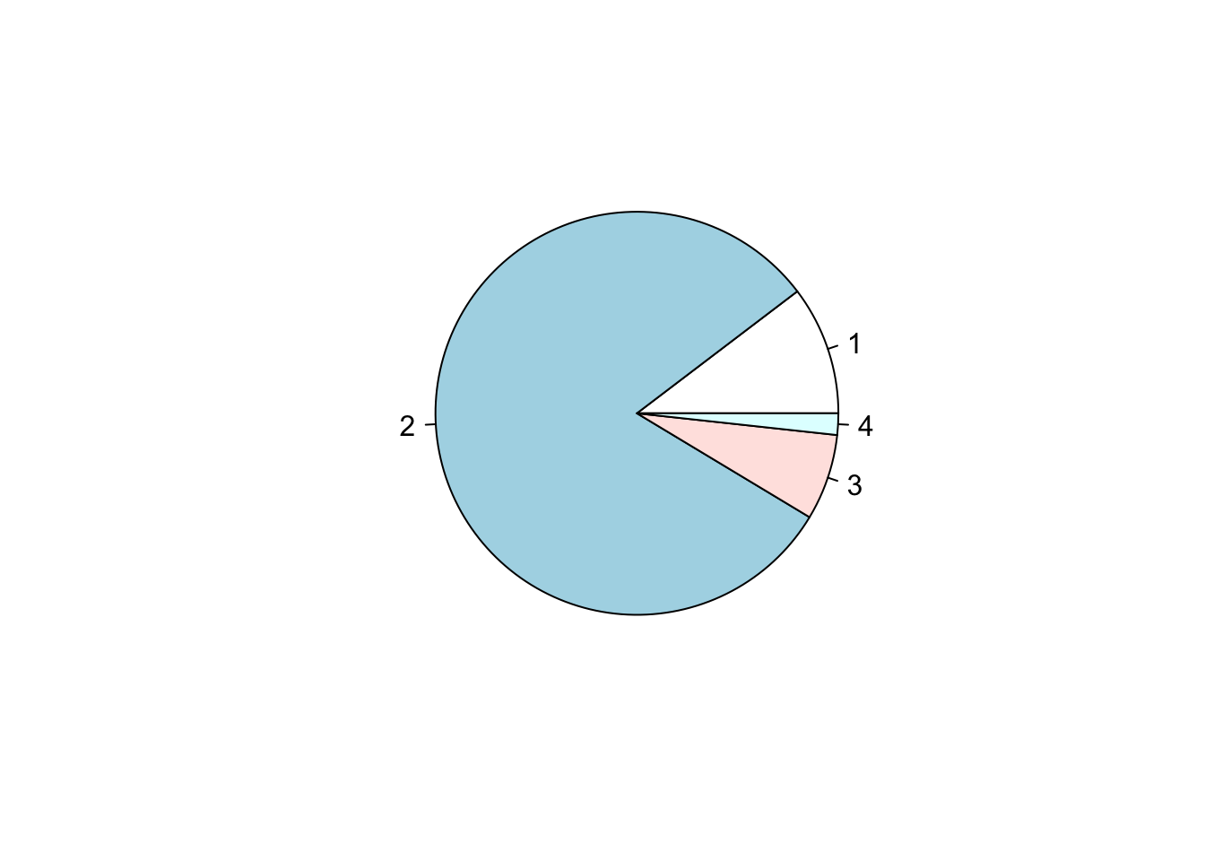
#Fully labelled Bar Plot
pie(counts, main="Piechart on OFSTED performance", labels=c("Outstanding (1)", "Good (2)", "Not Good (3)", "Bad (4)"))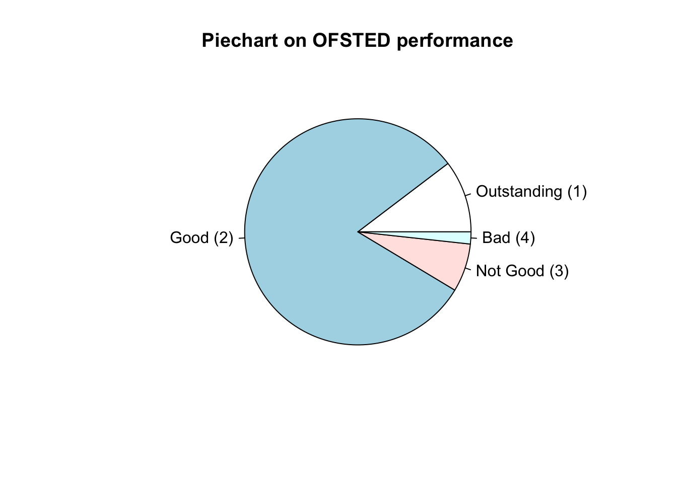
We can aggregate the number of students by performance to eyeball whether schools with more student perform either poorly or good on the OFSTED scale.
# aggregate the frequency of students from schools based of OfstedGrade in a table using the tapply()

totals <- tapply(SchoolData$TotalStudents, SchoolData$OfstedGrade, FUN=sum)
totals
## 1 2 3 4
## 3210 24225 1692 346#Fully labelled Bar Plot
barplot(totals, main="Student Distribution based on OFSTED performance", xlab ="OFSTED grades", ylab="Number of Primary Students in Ealing")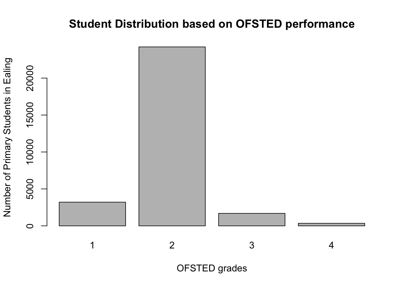
The OfstedGrade variable has classified schools according to the overall performance from 1 (outstanding) to 4 (poor). We can visual the frequency of schools by performance grade in a bar chart using barchart() function:
# tabulate the frequency of schools based on the OfstedGrade using table()
counts <- table(SchoolData$OfstedGrade)

# Pass the counts to the barplot() function & generate fully labelled Bar Plot
barplot(counts, main="School Distribution based on OFSTED performance", xlab ="OFSTED grades", ylab="Number of Schools")
1.9.4 Frequency Distributions
A frequency distribution table is a nice to way to perform a simple univariable analysis to summarize the number of schools (frequency) that have a set number of students within certain fixed ranges.
Let us gauge the minimum and maximum number of students, and create ranges between these two values.
## [1] 239## [1] 891We are going to create a new ranges column from 200 (based from lowest value i.e., 239) to 900 (i.e., based on the highest which is 891) to look something like 200-300, 301-400, 401-500, …, 801-900 by cutting the TotalStudents using the cut() function. This will help us to create the desired frequency distribution table in RStudio.
SchoolData$Ranges <- cut(SchoolData$TotalStudents, breaks=c(200, 300, 400, 500, 600, 700, 800, 900), labels = c("200-300","301-400","401-500","501-600","601-700","701-800","801-900"))Now, lets create the frequency table that shows the following: (1.) the frequency of schools with student numbers in those ranges; (2.) Cumulative frequency of schools; and (3.) proportions of schools falling in those ranges.
##
## 200-300 301-400 401-500 501-600 601-700 701-800 801-900
##       5       8      20      11       7       4       3
# now, add the cumulative frequency and proportion to get table output in RStudio
Output <- transform(freqtable, CumuFreq = cumsum(Freq), Proportions=prop.table(Freq))
# see final output
Output## Var1 Freq CumuFreq Proportions
## 1 200-300 5 5 0.08620690
## 2 301-400 8 13 0.13793103
## 3 401-500 20 33 0.34482759
## 4 501-600 11 44 0.18965517
## 5 601-700 7 51 0.12068966
## 6 701-800 4 55 0.06896552
## 7 801-900 3 58 0.05172414Above code shows you the rapid way of getting the frequency table. It only gives you the table though and there’s not decent way of getting the desired plots such as histogram and cumulative frequency plots because it involves of a lot of data wrangling…
Here is the complete code - the R-way for do this analysis.
Full Code
Let’s create the appropriate graphical outputs to accompany the frequency table. Just like how we created the ranges from 200 to 900 (of intervals 100). We can also use the seq() function. This generates a sequence of numbers (i.e., 200, 300, 400, 500, 600, 700, 800, 900) which we can also create the groupings:
## [1] 200 300 400 500 600 700 800 900We are going to use the cut() function slice up the TotalStudents column accordingly into the bins or groupings we created from the seq(). This should categorise the schools in Ealing based on the number of students into groups of 200-300, 301-400, 401-500, …, 801-900.
##  [1] (300,400] (300,400] (400,500] (600,700] (400,500] (400,500] (300,400]
##  [8] (500,600] (300,400] (200,300] (400,500] (400,500] (300,400] (400,500]
## [15] (600,700] (500,600] (500,600] (600,700] (400,500] (500,600] (200,300]
## [22] (500,600] (300,400] (400,500] (700,800] (500,600] (800,900] (800,900]
## [29] (500,600] (400,500] (800,900] (700,800] (600,700] (600,700] (500,600]
## [36] (400,500] (500,600] (200,300] (400,500] (700,800] (400,500] (600,700]
## [43] (400,500] (300,400] (300,400] (400,500] (400,500] (400,500] (200,300]
## [50] (600,700] (500,600] (500,600] (400,500] (400,500] (400,500] (700,800]
## [57] (200,300] (400,500]
## 7 Levels: (200,300] (300,400] (400,500] (500,600] (600,700] ... (800,900]
We going to generate the frequency table into a data frame and calculate components of our frequency table: i.e., frequency, relative frequency (or percentage), cumulative frequency and relative cumulative frequency all from the Group column:
#this creates the frequency tables
frequency_results <- data.frame(table(SchoolData$Groups))
#this renames the columns
colnames(frequency_results)[1] <- "Groups"
colnames(frequency_results)[2] <- "Frequency"
#this show the names of the columns
names(frequency_results)
## [1] "Groups" "Frequency"## Groups Frequency
## 1 (200,300] 5
## 2 (300,400] 8
## 3 (400,500] 20
## 4 (500,600] 11
## 5 (600,700] 7
## 6 (700,800] 4
## 7 (800,900] 3We got just the frequencies. Now, we to calculate the following: frequency, relative frequency (or percentage), cumulative frequency and relative cumulative frequency. The can be done as follows
# calculating the relative freq., cumulative freq., and cumulative relative frequency
frequency_results$RelativeFreq <- frequency_results$Frequency/sum(frequency_results$Frequency)
frequency_results$CumulativeFreq <- cumsum(frequency_results$Frequency)
frequency_results$CumulativeRelFreq <- cumsum(frequency_results$RelativeFreq)
Done! We can compute everything now… our complete frequency distribution table is:
##      Groups Frequency RelativeFreq CumulativeFreq CumulativeRelFreq
## 1 (200,300]         5   0.08620690              5         0.0862069
## 2 (300,400]         8   0.13793103             13         0.2241379
## 3 (400,500]        20   0.34482759             33         0.5689655
## 4 (500,600]        11   0.18965517             44         0.7586207
## 5 (600,700]         7   0.12068966             51         0.8793103
## 6 (700,800]         4   0.06896552             55         0.9482759
## 7 (800,900]         3   0.05172414             58         1.0000000
For our histogram, we use the hist() function to make one. Let us plot this and again use the xlab=, ylab= and main= arguments to label the graph and axes appropriately.
# histogram
hist(SchoolData$TotalStudents, breaks = classes,
    ylab="Frequency for schools",
    xlab="Total students",
    main= "Frequency Distribution of Schools in Ealing")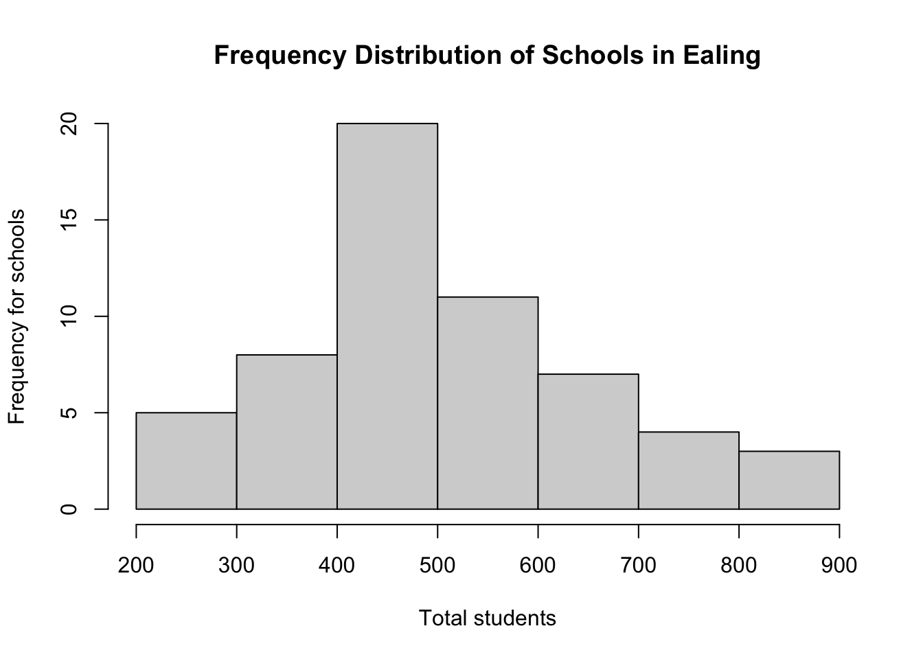
Lastly, we create the cumulative frequency plots.
# plot the cumulative frequency
# extract the cumulative frequency column
cumulative.freq0 <- c(0, frequency_results$CumulativeFreq)
cumulative.freq0
## [1] 0 5 13 33 44 51 55 58#create plot with classes values on x-axis and cumulative frequency values on y-axis
plot(classes, cumulative.freq0, main="Cumulative Frequency Distribution of Schools in Ealing" , xlab="Total Students", ylab="Cumulative Frequency: Schools")
#connect the dots to each point
lines(classes, cumulative.freq0)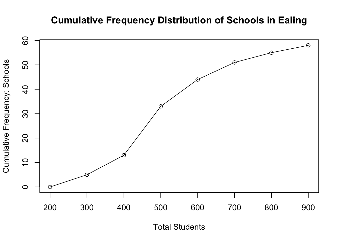
We also create the relative cumulative frequency plots.
# plot for relative cumulative frequency which is a cumulative percentage
# extract the relative cumulative frequency column
rel.cumulative.freq0 <- c(0, frequency_results$CumulativeRelFreq)
rel.cumulative.freq0
## [1] 0.0000000 0.0862069 0.2241379 0.5689655 0.7586207 0.8793103 0.9482759
## [8] 1.0000000#create plot with classes values on x-axis and cumulative frequency values on y-axis
plot(classes, rel.cumulative.freq0, main="Relative Cumulative Frequency Distribution of Schools in Ealing" , xlab="Total Students", ylab="Relative Cumulative Frequency [%]: Schools")
#connect the dots to each point
lines(classes, rel.cumulative.freq0)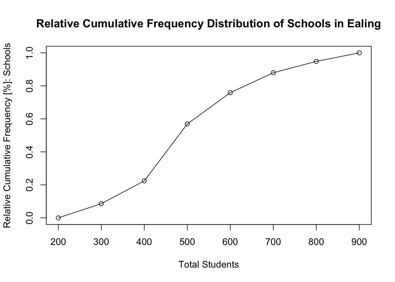
Interpretation: Out of the 58 primary schools in Ealing, 20 schools (0.3448 or 34.48%) have a student number totals ranging between 401-500 as the most frequent observation. The cumulative frequency of the range bracket for student numbers tells you how many schools have students from that range and lower. For instance 33 primary schools in Ealing have up to 500 students (which is 0.5689 or 56.89% of the data’s distribution).
Thoughts to self: cumsum() function… WTF man!?!
RECAP
This conclude practical tutorials for week 1. You can save your script by pressing the save button. To recap, in this section you have learnt how to:
Access R/RStudio Server and are familiar with RStudio’s environment
Creating a data frame, and loading a CSV file into R using
read.csv()Various basic functions for exploring the structure of a data frame, as well as how to subset data frame and manipulate columns to generate another.
We explored various ways for produce basic plots for discrete and categorical variables using
barplot()andpie()
1.10 Seminar tasks and questions
Please find the seminar task and seminar questions for this week’s seminar below.
Seminar Task : Use the seminar data set All Schools in London.csv and import it into RStudio. Perform the following tasks:
Create a column called
TotalStudentscontaining the total number of students for each schoolCreate a column called
PercentGirlswhich contains the estimated percentage of girls attending each school.Use the
tapply()function to calculate the total number of student by subgroup ortypeof school
Seminar Questions
Answer for following questions:
What are the names of schools that has the highest, and lowest number of students? [HINT: use
max(),min()andView()functions]Generate a fully labelled
barplot()and describe the distribution of schools by OFSTED scores.Explore the frequency of schools in London based on total number of students. Make a frequency table in R by creating the groups based on total students per school - starting from 0 to 2200, use the interval of 200 students to generate the groups as
0-200,201-400,401-600, …,2001-2200and hence number of schools falling into these groupings with these number of students. (Hint: see example in section 1.8.4. and make sure to use an appropriate interval for the ranges).
- Create a histogram.
- Create a cumulative frequency plot.
- Create a relative cumulative frequency plot.
- Provide an overall interpretation (see above example and those on slide #46 in Week 1’s lecture notes).
Important Note: The solution codes for this week will be released by the end of Thursday.