Week 4 Sourcing data

4.1 Introduction

Welcome to your fourth week of Introduction to Quantitative Research Methods. This week we will introduce you to sourcing and preparing data from official sources. For the tutorial we will apply what we have learnt over the past weeks onto a new secondary data set. OK… one final push to wrap the basic stuff covered today and previous weeks - LET’S DO THIS!

4.2 Sourcing data

Over the past weeks we have predominantly worked with two data sets that we provided for you: Ambulance and Assault Incidents data.csv and London historical population dataset.csv. Although these data sets are very useful to give you an introduction to Quantitative Research methods, in real life, you will probably have to source your own data. In the case of the social sciences, you often can find socioeconomic data on the websites of national statistical authorities such as the Office for National Statistics, United States Census Bureau, Statistics South Africa, or the National Bureau of Statistics of China. Also large international institutions like World Bank and Unicef compile socioeconomic data sets and make these available for research purposes. No matter where you will be getting your data from, however, you will have to know how to download and prepare these data sets in such a way that you can work with them in R to conduct your analysis.

Within the United Kingdom, the Office for National Statistics (ONS) is the largest producer of official statistics. ONS is responsible for collecting and publishing statistics related to the economy, population and society at national, regional and local levels. They are also responsible for conducting the census in England and Wales every 10 years (the census for Scotland and Northern Ireland are conducted by the National Records of Scotland and the Northern Ireland Statistics and Research Agency, respectively). Today we will be downloading a data set from ONS, prepare the data set as a csv file, and read our freshly created csv file into R.

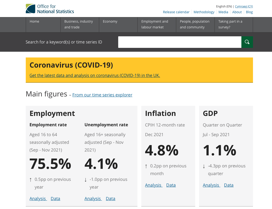
Figure 4.1: The website of the Office for National Statistics.

Because the population data in the London historical population dataset.csv we have been working with so far only goes as far as 2011, we will try to get some more recent population estimates on the ‘usual resident population’. Every year, ONS releases a new set of Middle Super Output Area mid-year population estimates. Currently, the latest available data set is that of mid-2019 and this is the data set that we are now going to download and prepare.

Note
The mid-year population estimates that we will be downloading are provided by ONS at the Middle Super Output Area (MSOA) level. MSOAs are one of the many administrative geographies that the ONS uses for reporting their small area statistics. An administrative geography is a way of dividing the country into smaller sub-divisions or areas that correspond with the area of responsibility of local authorities and government bodies. These geographies are updated as populations evolve and as a result, the boundaries of the administrative geographies are subject to either periodic or occasional change. The UK has quite a complex administrative geography, particularly due to having several countries within one overriding administration and then multiple ways of dividing the countries according to specific applications.

To download the data set, you need to take the following steps:

Step	Action
1	Navigate to the download page of the Middle Super Output Area population estimates: [Link]
2	Download the file `Mid-2020: SAPE23DT4` to your computer.
3	Because the file that you have now downloaded is a `zip` file, we first need to extract the file before we can use it. To unzip the file you can use the built-in functionality of your computer’s operating system. For Windows: right click on the `zip` file, select Extract All, and then follow the instructions. For Mac OS: double-click the `zip` file.
4	Open the file in Microsoft Excel or any other spreadsheet software. Please note that the instructions provided below use only cover Microsoft Excel.
5	Once opened your file should look similar as the screenshot in Figure 4.2.

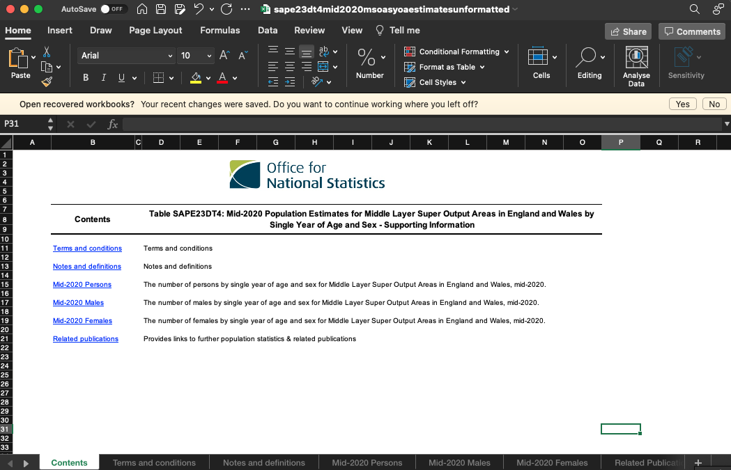
Figure 4.2: The Mid-2020: SAPE23DT4 file that we downloaded.

The download file will be in proper excel format .xlsx. The file name will look annoyingly look finicky: sape23dt4mid2020msoasyoaestimatesunformatted.xlsx. This is typical of an ONS data. The file probably does not look exactly like you thought it would because we do not directly see any data! In fact, ONS has put the data on different tabs. Some of these tabs contain the actual data, whilst others contain some meta-data and notes and definitions. The data that we want to use is found on the Mid-2020 Persons tab: the total number of people living in each MSOA. The problem we have now, however, is that the data as it is right now cannot be read into R without causing us lots of problems down the road. So even though we have the data we want to work with at our finger tips, we are not yet ready to read our data set into R! So, in video below, we will show you how to create a csv from the data that we want to use.

Follow the instructions for cleaning the data set manually. These are the steps that you need to take to turn the downloaded data into a csv:

Step	Action
1	Open the downloaded file in Microsoft Excel and activate the `Mid-2020 Persons` tab.
2	Highlight the columns: MSOA Code, MSOA Name, LA Code (2018 boundaries), LA name (2018 boundaries), LA Code (2020 boundaries), LA name (2020 boundaries), and All Ages. Do make sure that you do not include any of the whitespace or empty rows.
3	Scroll down all the way to the bottom of the file. Now hold down the shift button and click on the last value in the All Ages column. This value should be 9,722. All data should now be selected.
4	Now all the data that we need are selected we can copy them by right clicking and in the context menu opting for the copy option. Of course, you can also simply use `control` + `c` (Windows) or `command` + `c` (Mac OS).
5	Open a new, empty spreadsheet and paste the copied data into this new, empty spreadsheet. You can paste your copied data by right clicking on the first cell (A1) and in the context menu opting for the paste option. Of course, you can also simply use `control` + `v` (Windows) or `command` + `v` (Mac OS).
6	Conduct a visual check to make sure that you copied all the data.
7	Conduct a visual check to make sure that you did not copy any additional data.
8	Remove all formatting and make sure that empty columns are indeed empty.
9	Save this file as a `midyear2020.csv`. Make sure that you select `csv` as your file format (e.g. `CSV UTF8 (Comma-delimited) (.csv)`).
10	Inspect your data in a text editor such as Wordpad or Textedit to make sure the file you created is indeed a comma-separated file.

Now, for the moment of truth: let’s try and see if we can load our data into R! Of course, you will first need to upload your csv file to RStudio Server and set your working directory so that R can find the file - but you should be able to do that without any problems by now.

# load csv file from working directory
midyear <- read.csv('midyear2020.csv')

# inspect
midyear

Questions

Inspect the column names. Why do you think that they slightly differ from the ones that we saw in Microsoft Excel?
How many rows does the midyear dataframe have?
How many columns does the midyear dataframe have?

The column names may seem a little complicated but in fact simply refer to some of the administrative geographies that the ONS uses for their statistics. Don’t worry if you do not fully understand these as they are notoriously complicated and confusing!

Column heading	Full name	Description
MSOA.Code	MSOA Code	Middle Super Output Areas are one of the many administrative geographies that the ONS uses for reporting their small area statistics. These codes are used as a quick way of referring to them from official data sources.
MSOA.Name	MSOA Name	Name of the MSOA.
LA.Code..2018.boundaries	Local Authority District codes 2018	Local Authority Districts are a subnational division used for the purposes of local government. Each MSOA belongs to one Local Authority District, however, between years the boundaries of these Local Authority Districts sometimes change. These are the codes of the Local Authority District to which the MSOA belonged to in 2018.
LA.name..2018.boundaries	Local Authority District names 2018	Name of the Local Authority District to which the MSOA belonged to in 2018.
LA.Code..2020.boundaries	Local Authority District codes 2020	Code of the Local Authority District to which the MSOA belonged to in 2020
LA.name..2020.boundaries	Local Authority District names 2020	Name of the Local Authority District to which the MSOA belonged to in 2020.
All.Ages	Total number of people	The total number of people that is estimated to live in the MSOA mid-2020.

Now we at least have an idea about what our column names mean, we can rename them so that they are a little more intelligible and easier to work with in a later stage.

# rename columns
names(midyear) <- c('msoa_code','msoa_name','lad18_code','lad18_name','lad20_code','lad20_name','pop20')
# inspect
names(midyear)

## [1] "msoa_code"  "msoa_name"  "lad18_code" "lad18_name" "lad20_code"
## [6] "lad20_name" "pop20"

The write.csv() is the command we use to save our data.

# write to new csv, specify the object to be export out as a csv 'midyear' object
# next make sure to type the new name of the csv file to be named as: i.e., 'midyear2020_v2.csv'
write.csv(midyear, 'midyear2020_v2.csv', row.names=FALSE)

Great. This is all looking very good but we are not completely there yet. Now we sourced our data and managed to successfully read the data set into R, we will need to do conduct some final preparations so that our data is analysis ready.

Recap

In this section you have learnt how to:

Download data from the Office for National Statistics.
Select the data that you need and save these into a csv file.
Load the csv file that you created into R.

4.3 Preparing data

Even though the data set that we downloaded came from an official national statistical authority, the data is not directly ready for analysis. In fact, the vast majority of the data you will find in the public domain (or private domain for that matter) will be dirty data. With dirty data we mean data that needs some level of pre-processing, cleaning, and linkage before you can use it for your analysis. In the following, you will learn a consistent way to structure your data in R: tidy data. Tidy data, as formalised by R expert Hadley Wickham in his contribution to the Journal of Statistical Software is not only very much at the core of the tidyverse R package that we will introduce you to, but also of general importance when organising your data.

As you know by now, your basic R functionality (the base package) can be extended by installing additional packages. These packages are the fundamental units of reproducible R code and include functions, documentation, and sample data. Last week, we introduced you to the ggplot2 package: a general scheme for data visualisation that breaks up graphs into semantic components such as scales and layers. Today we will introduce you to the tidyverse package. This package is specifically created to make working with data, including data cleaning and data preparation, easier. Let’s start by installing the tidyverse package using the install_packages() function in the same way as we installed the ggplot2 package last week.

Install tidyverse package using the install_packages() function now.

Note
The tidyverse package is in fact a collection of packages that are specifically designed for data science tasks. Where in many cases different packages work all slightly differently, all packages of the tidyverse share the underlying design philosophy, grammar, and data structures. The ggplot2 package that you worked with last week is actually one of the core package of the tidyverse. This also means that if you load the tidyverse package through library(tidyverse) you directly have access to all the functions that are part of the ggplot2 package and you do not have to load the ggplot2 package separately. Because the tidyverse consists of multiple packages, it may take a little while before everything is installed so be patient! For more information on tidyverse, have a look at https://www.tidyverse.org/.

If your installation was successful, you can now load the tidyverse as follows:

# load the tidyverse 
library(tidyverse)

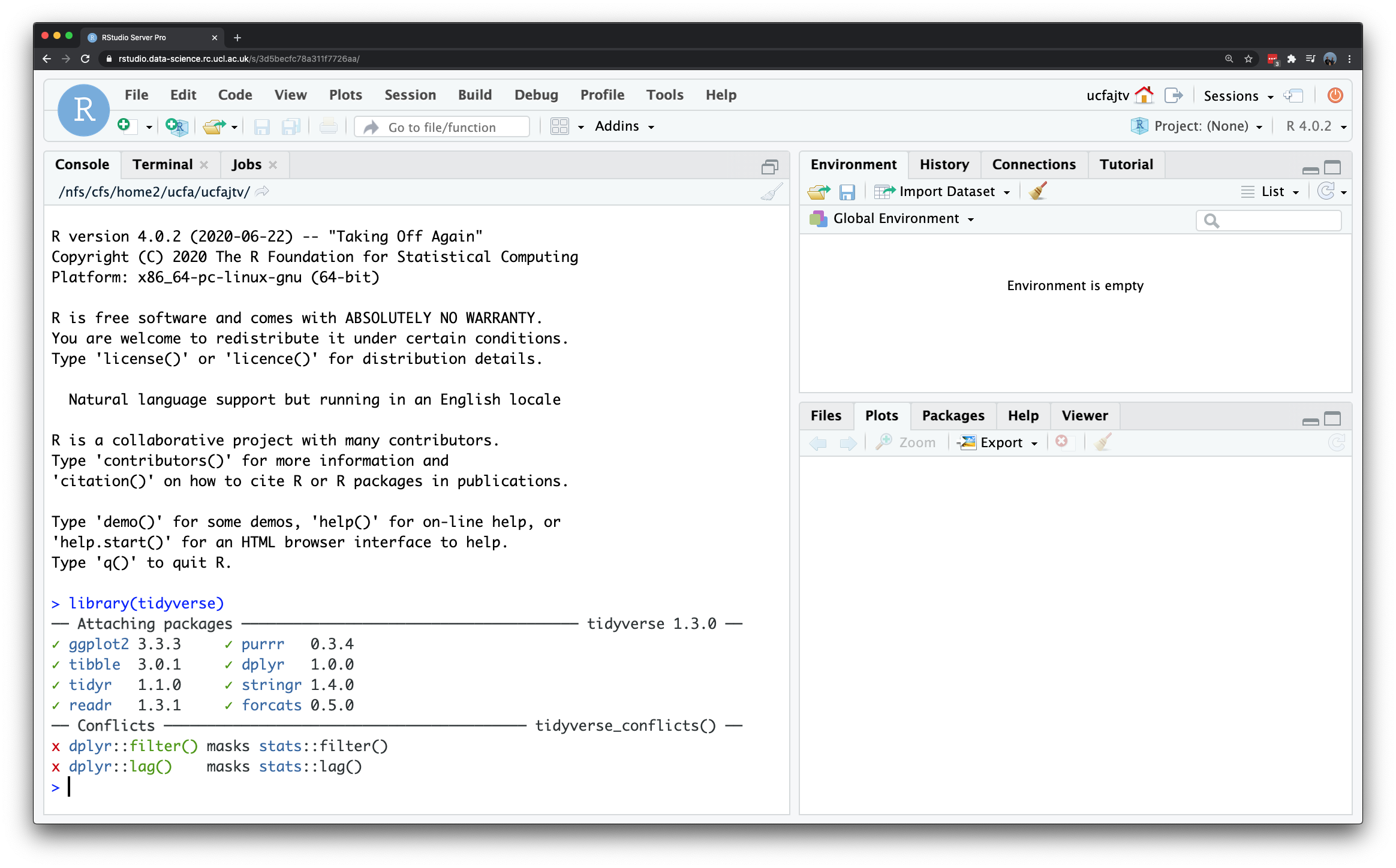
Figure 4.3: Loading the tidyverse.

Note
After loading the tidyverse, you may get a short information messages to inform you which packages are attached to your R session and whether there are any conflicting functions. This simply means that there are functions that are named the same across the packages that you have loaded. For instance, when you load the tidyverse in a fresh R session, the tidyverse will tell you that two functions from the dplyr package (which is an integral part of the tidyverse package) mask the functionality of two functions of the stats package (which is part of base R). This simply means that if you now type in filter() you will get the dplyr functionality and not the functionality of the stats. This is very important information as both these functions do something completely different! You can still use the filter() function from the stats package but then you have to explicitly tell R that you want to use the function called filter() within the stats package: stats::filter().

Now that we have loaded the tidyverse we can continue with our data preparation. We will start by reading in the csv file that we created earlier, however, we will use the function read_csv() from the tidyverse instead of the function read.csv() from base R. The function read_csv returns a so-called tibble. Tibbles are data frames, but they tweak some older behaviours to make life a little easier.

# load csv file from working directory
midyear <- read_csv('midyear2020_v2.csv')

# inspect
midyear

## # A tibble: 7,201 × 7
##    msoa_code msoa_name      lad18_code lad18_name lad20_code lad20_name pop20
##    <chr>     <chr>          <chr>      <chr>      <chr>      <chr>      <dbl>
##  1 E02002483 Hartlepool 001 E06000001  Hartlepool E06000001  Hartlepool 10332
##  2 E02002484 Hartlepool 002 E06000001  Hartlepool E06000001  Hartlepool 10440
##  3 E02002485 Hartlepool 003 E06000001  Hartlepool E06000001  Hartlepool  8165
##  4 E02002487 Hartlepool 005 E06000001  Hartlepool E06000001  Hartlepool  5174
##  5 E02002488 Hartlepool 006 E06000001  Hartlepool E06000001  Hartlepool  5894
##  6 E02002489 Hartlepool 007 E06000001  Hartlepool E06000001  Hartlepool  7638
##  7 E02002490 Hartlepool 008 E06000001  Hartlepool E06000001  Hartlepool  6182
##  8 E02002491 Hartlepool 009 E06000001  Hartlepool E06000001  Hartlepool  6450
##  9 E02002492 Hartlepool 010 E06000001  Hartlepool E06000001  Hartlepool  6895
## 10 E02002493 Hartlepool 011 E06000001  Hartlepool E06000001  Hartlepool  6722
## # … with 7,191 more rows

Questions

Do you notice a difference between how base R prints a data frame and how a tibble gets printed?

Let’s have a better look at our data particularly the data types. We can can do this through the str() function:

# inspect
str(midyear)

## spc_tbl_ [7,201 × 7] (S3: spec_tbl_df/tbl_df/tbl/data.frame)
##  $ msoa_code : chr [1:7201] "E02002483" "E02002484" "E02002485" "E02002487" ...
##  $ msoa_name : chr [1:7201] "Hartlepool 001" "Hartlepool 002" "Hartlepool 003" "Hartlepool 005" ...
##  $ lad18_code: chr [1:7201] "E06000001" "E06000001" "E06000001" "E06000001" ...
##  $ lad18_name: chr [1:7201] "Hartlepool" "Hartlepool" "Hartlepool" "Hartlepool" ...
##  $ lad20_code: chr [1:7201] "E06000001" "E06000001" "E06000001" "E06000001" ...
##  $ lad20_name: chr [1:7201] "Hartlepool" "Hartlepool" "Hartlepool" "Hartlepool" ...
##  $ pop20     : num [1:7201] 10332 10440 8165 5174 5894 ...
##  - attr(*, "spec")=
##   .. cols(
##   ..   msoa_code = col_character(),
##   ..   msoa_name = col_character(),
##   ..   lad18_code = col_character(),
##   ..   lad18_name = col_character(),
##   ..   lad20_code = col_character(),
##   ..   lad20_name = col_character(),
##   ..   pop20 = col_double()
##   .. )
##  - attr(*, "problems")=<externalptr>

The output of the str() function tells us that every column in our data frame (tibble) is of type “character”, which comes down to a variable that contains textual data. What is interesting, obviously, is that also our pop20 variable is considered a character variable. The reason for this is that in the original data white space is used as thousands separator (i.e. 11 000 instead of 11000 or 11,000). Does it matter? Well, let’s try to calculate the mean and median of our pop20 variable:

# mean
mean(midyear$pop20)

## [1] 8293.254

# median
median(midyear$pop20)

## [1] 7974

Note
Depending on computer settings and the version of Microsoft Excel or spreadsheet software that you use, in some case you could get a numeric variable (e.g. double) instead of a character variable for your pop120 variable. If so: you are lucky and do not need to undertake the steps below to turn this character column into a numeric column. (This will also mean that at this stage your results will differ from the results shown here.) Just continue with the tutorial by carefully reading through the steps that you would have needed to take if indeed your results would have been the same as shown here.

As you can see, this is not working perfectly for the simple fact that the the mean() function requires a numeric variable as its input! The median() does return a value, however, this is not per se the median that we are interested in as the sorting of the data is now done alphabetically: see for your self what happens when using the sort() function on the pop20 variable. Fortunately, there are some functions in the dplyr package, which is part of the tidyverse, that will help us further cleaning and preparing our data. Some of the most important and useful functions are:

Package	Function	Use to
dplyr	select	select columns
dplyr	filter	select rows
dplyr	mutate	transform or recode variables
dplyr	summarise	summarise data
dplyr	group by	group data into subgroups for further processing

Note
Remember that when you encounter a function in a piece of R code that you have not seen before and you are wondering what it does that you can get access the documentation through ?name_of_function, e.g. ?mutate. For almost any R package, the documentation contains a list of arguments that the function takes, in which format the functions expects these arguments, as well as a set of usage examples.

Let’s have a look at two of the dplyr functions: select() and filter().

# select columns with the select function
# note that within dplyr we not use quotation marks to refer to columns
midyear_sel <- select(midyear,msoa_code,msoa_name,lad20_code,lad20_name,pop20)
# inspect
midyear_sel

## # A tibble: 7,201 × 5
##    msoa_code msoa_name      lad20_code lad20_name pop20
##    <chr>     <chr>          <chr>      <chr>      <dbl>
##  1 E02002483 Hartlepool 001 E06000001  Hartlepool 10332
##  2 E02002484 Hartlepool 002 E06000001  Hartlepool 10440
##  3 E02002485 Hartlepool 003 E06000001  Hartlepool  8165
##  4 E02002487 Hartlepool 005 E06000001  Hartlepool  5174
##  5 E02002488 Hartlepool 006 E06000001  Hartlepool  5894
##  6 E02002489 Hartlepool 007 E06000001  Hartlepool  7638
##  7 E02002490 Hartlepool 008 E06000001  Hartlepool  6182
##  8 E02002491 Hartlepool 009 E06000001  Hartlepool  6450
##  9 E02002492 Hartlepool 010 E06000001  Hartlepool  6895
## 10 E02002493 Hartlepool 011 E06000001  Hartlepool  6722
## # … with 7,191 more rows

# filter rows with the filter function
# note that within dplyr we not use quotation marks to refer to columns
midyear_fil <- filter(midyear,lad20_name=='Leeds')
# inspect
midyear_fil

## # A tibble: 107 × 7
##    msoa_code msoa_name lad18_code lad18_name lad20_code lad20_name pop20
##    <chr>     <chr>     <chr>      <chr>      <chr>      <chr>      <dbl>
##  1 E02002330 Leeds 001 E08000035  Leeds      E08000035  Leeds       6663
##  2 E02002331 Leeds 002 E08000035  Leeds      E08000035  Leeds       7082
##  3 E02002332 Leeds 003 E08000035  Leeds      E08000035  Leeds       6202
##  4 E02002333 Leeds 004 E08000035  Leeds      E08000035  Leeds       7553
##  5 E02002334 Leeds 005 E08000035  Leeds      E08000035  Leeds       7160
##  6 E02002335 Leeds 006 E08000035  Leeds      E08000035  Leeds       7460
##  7 E02002336 Leeds 007 E08000035  Leeds      E08000035  Leeds       6585
##  8 E02002337 Leeds 008 E08000035  Leeds      E08000035  Leeds       7392
##  9 E02002338 Leeds 009 E08000035  Leeds      E08000035  Leeds       6769
## 10 E02002339 Leeds 010 E08000035  Leeds      E08000035  Leeds       5297
## # … with 97 more rows

Questions

How can we get the same data frame with selected columns (midyear_sel) using the base R syntax we have been using in previous weeks?
How can we get the same data frame with filtered rows (midyear_fil) using the base R syntax we have been using in previous weeks?

With the mutate() function we can easily create new columns, so let’s try this function to see if we can create a new variable that contains all the data from pop20 in a numeric format.

# create a new variable named pop19_no space
# by replacing all white space with nothing using the "str_replace_all" function
midyear <- mutate(midyear, pop20_nospace=str_replace_all(pop20, pattern=' ', repl=''))
# inspect
midyear

## # A tibble: 7,201 × 8
##    msoa_code msoa_name      lad18_code lad18_name lad20_…¹ lad20…² pop20 pop20…³
##    <chr>     <chr>          <chr>      <chr>      <chr>    <chr>   <dbl> <chr>  
##  1 E02002483 Hartlepool 001 E06000001  Hartlepool E060000… Hartle… 10332 10332  
##  2 E02002484 Hartlepool 002 E06000001  Hartlepool E060000… Hartle… 10440 10440  
##  3 E02002485 Hartlepool 003 E06000001  Hartlepool E060000… Hartle…  8165 8165   
##  4 E02002487 Hartlepool 005 E06000001  Hartlepool E060000… Hartle…  5174 5174   
##  5 E02002488 Hartlepool 006 E06000001  Hartlepool E060000… Hartle…  5894 5894   
##  6 E02002489 Hartlepool 007 E06000001  Hartlepool E060000… Hartle…  7638 7638   
##  7 E02002490 Hartlepool 008 E06000001  Hartlepool E060000… Hartle…  6182 6182   
##  8 E02002491 Hartlepool 009 E06000001  Hartlepool E060000… Hartle…  6450 6450   
##  9 E02002492 Hartlepool 010 E06000001  Hartlepool E060000… Hartle…  6895 6895   
## 10 E02002493 Hartlepool 011 E06000001  Hartlepool E060000… Hartle…  6722 6722   
## # … with 7,191 more rows, and abbreviated variable names ¹lad20_code,
## #   ²lad20_name, ³pop20_nospace

# create a new variable named pop20_numeric
# by transforming the pop20_nospace variable using the "as.numeric" function
midyear <- mutate(midyear,pop20_numeric=as.numeric(pop20_nospace))
# inspect
midyear

## # A tibble: 7,201 × 9
##    msoa_code msoa_name     lad18…¹ lad18…² lad20…³ lad20…⁴ pop20 pop20…⁵ pop20…⁶
##    <chr>     <chr>         <chr>   <chr>   <chr>   <chr>   <dbl> <chr>     <dbl>
##  1 E02002483 Hartlepool 0… E06000… Hartle… E06000… Hartle… 10332 10332     10332
##  2 E02002484 Hartlepool 0… E06000… Hartle… E06000… Hartle… 10440 10440     10440
##  3 E02002485 Hartlepool 0… E06000… Hartle… E06000… Hartle…  8165 8165       8165
##  4 E02002487 Hartlepool 0… E06000… Hartle… E06000… Hartle…  5174 5174       5174
##  5 E02002488 Hartlepool 0… E06000… Hartle… E06000… Hartle…  5894 5894       5894
##  6 E02002489 Hartlepool 0… E06000… Hartle… E06000… Hartle…  7638 7638       7638
##  7 E02002490 Hartlepool 0… E06000… Hartle… E06000… Hartle…  6182 6182       6182
##  8 E02002491 Hartlepool 0… E06000… Hartle… E06000… Hartle…  6450 6450       6450
##  9 E02002492 Hartlepool 0… E06000… Hartle… E06000… Hartle…  6895 6895       6895
## 10 E02002493 Hartlepool 0… E06000… Hartle… E06000… Hartle…  6722 6722       6722
## # … with 7,191 more rows, and abbreviated variable names ¹lad18_code,
## #   ²lad18_name, ³lad20_code, ⁴lad20_name, ⁵pop20_nospace, ⁶pop20_numeric

# inspect
str(midyear)

## tibble [7,201 × 9] (S3: tbl_df/tbl/data.frame)
##  $ msoa_code    : chr [1:7201] "E02002483" "E02002484" "E02002485" "E02002487" ...
##  $ msoa_name    : chr [1:7201] "Hartlepool 001" "Hartlepool 002" "Hartlepool 003" "Hartlepool 005" ...
##  $ lad18_code   : chr [1:7201] "E06000001" "E06000001" "E06000001" "E06000001" ...
##  $ lad18_name   : chr [1:7201] "Hartlepool" "Hartlepool" "Hartlepool" "Hartlepool" ...
##  $ lad20_code   : chr [1:7201] "E06000001" "E06000001" "E06000001" "E06000001" ...
##  $ lad20_name   : chr [1:7201] "Hartlepool" "Hartlepool" "Hartlepool" "Hartlepool" ...
##  $ pop20        : num [1:7201] 10332 10440 8165 5174 5894 ...
##  $ pop20_nospace: chr [1:7201] "10332" "10440" "8165" "5174" ...
##  $ pop20_numeric: num [1:7201] 10332 10440 8165 5174 5894 ...

Note the information for pop20_numeric: str indicates that the column is now of type num (i.e. numeric). This is much better. We can now try to calculate the median and the mean again:

# calculate the mean of the pop19_numeric variable
mean(midyear$pop20_numeric)

## [1] 8293.254

# calculate the median of the pop19_numeric variable
median(midyear$pop20_numeric)

## [1] 7974

Everything seems to be working fine now and our data is now finally ready for analysis, so it is probably wise to save’s save it.

# write to new csv
write.csv(midyear, 'midyear2020_clean.csv', row.names=FALSE)

Recap

In this section you have learnt how to:

Transform your data frame to a tibble.
Use some of the functionality of the tidyverse to prepare your data set and make it suitable for analysis.

4.4 Seminar

Please find the seminar task and seminar questions for this week’s seminar below.

Note
Please make sure that you have executed the seminar task and have answered the seminar questions before the seminar!

Seminar task

Of course, we did not go through all the trouble of downloading and preparing this file without using it. Use the cleaned version of the midyear data set that we just created to:

Create a new object / data set that only contains data for the Local Authority District (2020 boundaries) of Manchester.
Create a new object / data set that only contains data for the Local Authority District (2020 boundaries) of Birmingham.

For both new objects:

Calculate the mean, median, and standard deviation of the pop20_numeric variable.
Create a boxplot of the pop20_numeric variable using the ggplot2 package.
Create a histogram of the pop20_numeric variable using the ggplot2 package. Select a bin width that you think is appropriate.

Seminar questions

Compare the results of the descriptive statistics you have calculated for your Birmingham object / data set with the results of the descriptive statistics you have calculated for you Manchester data set. What do these descriptive statistics tell you?
Why did you select the bin width that you used for creating your histograms?
Compare the histograms that you created for your Birmingham object / data set and the Manchester data set, what can you tell about the population distribution of both Local Authority Districts?

Additional tasks (in your own time)

If you found these assignments and questions relatively easy and want an assignment that is a little more realistic, try to do the following:

Download the mid-year population estimates for 2018 to your computer (Mid-2018: SAPE21DT4 (unformatted)). Make sure that you download the file with exactly this name: it is listed under the “supporting files you may find useful” heading.
Prepare a csv file of the first three columns of the Mid-2018 Perons tab and import into R.
Give the columns the following names: msoa_code, msoa_name, pop18.
Take the necessary steps in R to make sure that all numeric variables are also recognised by R as numeric variables.
Join the 2018 and 2019 midyear population data set by using the left join() function from the tidyverse() package, e.g. something like: midyear <- left_join(midyear2018, midyear2019, by=c('msoa_code'='msoa_code').
Calculate the population change between 2018 and 2019.
Create a histogram of the population change.
Which MSOA has the largest decline in population between 2018 and 2019? Which MSOA had the largest increase in population between 2018 and 2019?