Bonus Content: Creating tables in RStudio
This is a bonus section and so its entirely optional which can be studied at your own time. We are basically going to show you how to code out a table from RStudio to save you a lot time and energy, as well as potential grief with doing this in Microsoft Word.
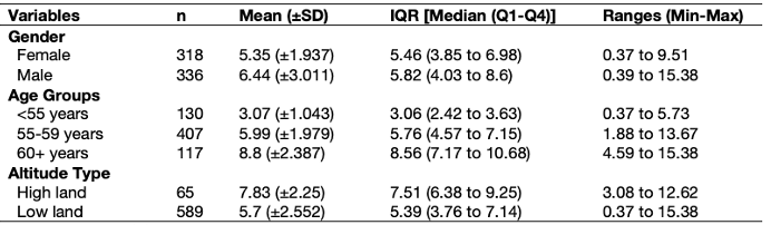
Overall summary table by categorical variables
Remember this table in Week 2’s lecture (see slide 42 and 44)?
We are going to use the dataset Health Data.csv. Download it by clicking this link [HERE]
We are producing an overall summary of the lung capacity volume (LCV) which is broken down by the following categorical characteristics: gender, age groups and altitude type.
You can use the dplyr package to compute the desired summary statistics accordingly by the categories using the group_by() and summarize() functions. We will try this for gender first.
# loading package for 'dplyr'
library("dplyr")

# import the health dataset
dataset.eg <- read.csv("Health Data.csv")

# this code churns out the summary statistics for gender only
# in the summarize() make it report n, mean, sd, median, quantiles and min and max
# store first part of result in object called `gender_table`
gender_table <-
    dataset.eg %>%
    group_by(gender) %>%
    summarize(n = length(initialLCV), mean = mean(initialLCV), sd = sd(initialLCV),
        median = median(initialLCV), q1 = quantile(initialLCV, 0.25), q3 = quantile(initialLCV, 0.75),
        min = min(initialLCV), max = max(initialLCV))

# show result for gender
gender_table
This the result for gender:
> gender_table
# A tibble: 2 × 9
  gender     n  mean    sd median    q1    q3   min   max
  <chr>  <int> <dbl> <dbl>  <dbl> <dbl> <dbl> <dbl> <dbl>
1 female   318  5.35  1.94   5.46  3.85  6.98 0.373  9.51
2 male     336  6.44  3.01   5.82  4.03  8.60 0.388 15.4
You can view the result as a data frame by running the code View(gender_table).
Now, we can repeat this for the age groups and altitude type variables:
ageg_table <-
    dataset.eg %>%
    group_by(agegroup) %>%
    summarize(n = length(initialLCV), mean = mean(initialLCV), sd = sd(initialLCV),
        median = median(initialLCV), q1 = quantile(initialLCV, 0.25), q3 = quantile(initialLCV, 0.75),
        min = min(initialLCV), max = max(initialLCV))

altitude_table <-
    dataset.eg %>%
    group_by(altitude) %>%
    summarize(n = length(initialLCV), mean = mean(initialLCV), sd = sd(initialLCV),
        median = median(initialLCV), q1 = quantile(initialLCV, 0.25), q3 = quantile(initialLCV, 0.75),
        min = min(initialLCV), max = max(initialLCV))

# view results
ageg_table
altitude_table
See results for the age groups and altitude:
> ageg_table
# A tibble: 3 × 9
  agegroup        n  mean    sd median    q1    q3   min   max
  <chr>       <int> <dbl> <dbl>  <dbl> <dbl> <dbl> <dbl> <dbl>
1 <55 years     130  3.07  1.04   3.06  2.42  3.63 0.373  5.73
2 55-59 years   407  5.99  1.98   5.76  4.57  7.15 1.88  13.7
3 60+ years     117  8.80  2.39   8.56  7.17 10.7  4.59  15.4

> altitude_table
# A tibble: 2 × 9
  altitude      n  mean    sd median    q1    q3   min   max
  <chr>     <int> <dbl> <dbl>  <dbl> <dbl> <dbl> <dbl> <dbl>
1 high land    65  7.83  2.25   7.51  6.38  9.25 3.08   12.6
2 low land    589  5.70  2.55   5.40  3.76  7.14 0.373  15.4
Before appending the tables together, in each table - i.e., gender_table, ageg_table and altitude_table, we will need to change the name of the first column to something consist across all tables for the appendage to work.
# change the first column name to something like `varname_cat`
colnames(ageg_table)[1] <- "varname_cat"
colnames(gender_table)[1] <- "varname_cat"
colnames(altitude_table)[1] <- "varname_cat"
Next step is to append the tables using rbind() in the order of gender_table, ageg_table and altitude_table.
# stitch tables together using rbind()
descriptive.table <- rbind(gender_table, ageg_table, altitude_table)

# view output
descriptive.table
The result looks something like:
> descriptive.table
# A tibble: 7 × 9
  varname_cat     n  mean    sd median    q1    q3   min   max
  <chr>       <int> <dbl> <dbl>  <dbl> <dbl> <dbl> <dbl> <dbl>
1 female        318  5.35  1.94   5.46  3.85  6.98 0.373  9.51
2 male          336  6.44  3.01   5.82  4.03  8.60 0.388 15.4
3 <55 years     130  3.07  1.04   3.06  2.42  3.63 0.373  5.73
4 55-59 years   407  5.99  1.98   5.76  4.57  7.15 1.88  13.7
5 60+ years     117  8.80  2.39   8.56  7.17 10.7  4.59  15.4
6 high land      65  7.83  2.25   7.51  6.38  9.25 3.08  12.6
7 low land      589  5.70  2.55   5.40  3.76  7.14 0.373 15.4
Now, fun part - we need to bring the mean and standard deviation estimates into one column. In the same vein, we want the median and Q1 and Q3 results in one column, as well as the ranged values for minimum and maximum both to be in one column.
We can generate new columns within that descriptive.table object and use the paste() to render the results as a text string which can be pasted to the way see fit! You examine at the code carefully
# create a new column for mean and sd - paste items as 3.56 (±2.23)
descriptive.table$mean_sd <- paste(round(descriptive.table$mean, 2), " (±", round(descriptive.table$sd, 3), ")", sep = "")
# create a new column for median, q1 and q3 - paste items as 3.56 (1.23 to 5.63)
descriptive.table$IQR <- paste(round(descriptive.table$median, 2), " (", round(descriptive.table$q1, 2), " to ", round(descriptive.table$q3, 2), ")", sep = "")
# create a new column for min and max - paste items as 3.56 to 14.59
descriptive.table$Range <- paste(round(descriptive.table$min, 2), " to ", round(descriptive.table$max, 2), sep = "")

# see table
descriptive.table
Look at the later columns:
> descriptive.table
# A tibble: 7 × 12
  varname_cat     n  mean    sd median    q1    q3   min   max mean_sd       IQR                  Range
  <chr>       <int> <dbl> <dbl>  <dbl> <dbl> <dbl> <dbl> <dbl> <chr>         <chr>                <chr>
1 female        318  5.35  1.94   5.46  3.85  6.98 0.373  9.51 5.35 (±1.937) 5.46 (3.85 to 6.98)  0.37 to 9.51
2 male          336  6.44  3.01   5.82  4.03  8.60 0.388 15.4  6.44 (±3.011) 5.82 (4.03 to 8.6)   0.39 to 15.38
3 <55 years     130  3.07  1.04   3.06  2.42  3.63 0.373  5.73 3.07 (±1.043) 3.06 (2.42 to 3.63)  0.37 to 5.73
4 55-59 years   407  5.99  1.98   5.76  4.57  7.15 1.88  13.7  5.99 (±1.979) 5.76 (4.57 to 7.15)  1.88 to 13.67
5 60+ years     117  8.80  2.39   8.56  7.17 10.7  4.59  15.4  8.8 (±2.387)  8.56 (7.17 to 10.68) 4.59 to 15.38
6 high land      65  7.83  2.25   7.51  6.38  9.25 3.08  12.6  7.83 (±2.25)  7.51 (6.38 to 9.25)  3.08 to 12.62
7 low land      589  5.70  2.55   5.40  3.76  7.14 0.373 15.4  5.7 (±2.552)  5.39 (3.76 to 7.14)  0.37 to 15.38
Now, discard redundant columns and only retain these pasted ones:
table_breakdown_by_cat <- descriptive.table[,c(1, 2, 10, 11, 12)]

# see final table
table_breakdown_by_cat
We have obtained the desired table:
> table_breakdown_by_cat
# A tibble: 7 × 5
  varname_cat     n mean_sd       IQR                  Range
  <chr>       <int> <chr>         <chr>                <chr>
1 female        318 5.35 (±1.937) 5.46 (3.85 to 6.98)  0.37 to 9.51
2 male          336 6.44 (±3.011) 5.82 (4.03 to 8.6)   0.39 to 15.38
3 <55 years     130 3.07 (±1.043) 3.06 (2.42 to 3.63)  0.37 to 5.73
4 55-59 years   407 5.99 (±1.979) 5.76 (4.57 to 7.15)  1.88 to 13.67
5 60+ years     117 8.8 (±2.387)  8.56 (7.17 to 10.68) 4.59 to 15.38
6 high land      65 7.83 (±2.25)  7.51 (6.38 to 9.25)  3.08 to 12.62
7 low land      589 5.7 (±2.552)  5.39 (3.76 to 7.14)  0.37 to 15.38
This is how you make such tables in RStudio. Now, its all about exporting it to a spreadsheet, and copying and pasting it to Microsoft Word document where you can apply the cosmetic changes to make the table publication-worthy. Make sure that the code is indeed churning out the correct information.
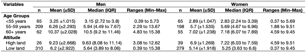
Summary table by categorical variables further stratified
Do you also remember this table in Week 2’s lecture (see slide 43)?
This is the full code for create that table:
# overall but broken by a specific categorical variable
# keep female only
dataset.eg_female <- dataset.eg[dataset.eg$gender=="female",]
# keep male only
dataset.eg_male <- dataset.eg[dataset.eg$gender=="male",]

# create a table for female only
ageg_table.fe <-
    dataset.eg_female %>%
    group_by(agegroup) %>%
    summarize(n = length(initialLCV), mean = mean(initialLCV), sd = sd(initialLCV),
        median = median(initialLCV), q1 = quantile(initialLCV, 0.25), q3 = quantile(initialLCV, 0.75),
        min = min(initialLCV), max = max(initialLCV))

altitude_table.fe <-
    dataset.eg_female %>%
    group_by(altitude) %>%
    summarize(n = length(initialLCV), mean = mean(initialLCV), sd = sd(initialLCV),
        median = median(initialLCV), q1 = quantile(initialLCV, 0.25), q3 = quantile(initialLCV, 0.75),
        min = min(initialLCV), max = max(initialLCV))

colnames(ageg_table.fe)[1] <- "varname_cat"
colnames(altitude_table.fe)[1] <- "varname_cat"

descriptive.table.fe <- rbind(ageg_table.fe, altitude_table.fe)

descriptive.table.fe$mean_sd.fe <- paste(round(descriptive.table.fe$mean, 2), " (±", round(descriptive.table.fe$sd, 3), ")", sep = "")
descriptive.table.fe$IQR.fe <- paste(round(descriptive.table.fe$median, 2), " (", round(descriptive.table.fe$q1, 2), " to ", round(descriptive.table.fe$q3, 2), ")", sep = "")
descriptive.table.fe$Range.fe <- paste(round(descriptive.table.fe$min, 2), " to ", round(descriptive.table.fe$max, 2), sep = "")

table_breakdown_by_cat.fe <- descriptive.table.fe[,c(1, 2, 10, 11, 12)]

# create a table for male only
ageg_table.ma <-
    dataset.eg_male %>%
    group_by(agegroup) %>%
    summarize(n = length(initialLCV), mean = mean(initialLCV), sd = sd(initialLCV),
        median = median(initialLCV), q1 = quantile(initialLCV, 0.25), q3 = quantile(initialLCV, 0.75),
        min = min(initialLCV), max = max(initialLCV))

altitude_table.ma <-
    dataset.eg_male %>%
    group_by(altitude) %>%
    summarize(n = length(initialLCV), mean = mean(initialLCV), sd = sd(initialLCV),
        median = median(initialLCV), q1 = quantile(initialLCV, 0.25), q3 = quantile(initialLCV, 0.75),
        min = min(initialLCV), max = max(initialLCV))

colnames(ageg_table.ma)[1] <- "varname_cat"
colnames(altitude_table.ma)[1] <- "varname_cat"

descriptive.table.ma <- rbind(ageg_table.ma, altitude_table.ma)

descriptive.table.ma$mean_sd.ma <- paste(round(descriptive.table.ma$mean, 2), " (±", round(descriptive.table.ma$sd, 3), ")", sep = "")
descriptive.table.ma$IQR.ma <- paste(round(descriptive.table.ma$median, 2), " (", round(descriptive.table.ma$q1, 2), " to ", round(descriptive.table.ma$q3, 2), ")", sep = "")
descriptive.table.ma$Range.ma <- paste(round(descriptive.table.ma$min, 2), " to ", round(descriptive.table.ma$max, 2), sep = "")

table_breakdown_by_cat.ma <- descriptive.table.ma[,c(1, 2, 10, 11, 12)]

# merge the table_breakdown_by_cat.ma and table_breakdown_by_cat.fe to produce the table in slide 43
table_breakdown_cat_gender <- merge(table_breakdown_by_cat.ma, table_breakdown_by_cat.fe,
    by.x = "varname_cat", by.y = "varname_cat")

# View output table
table_breakdown_cat_gender
Show table:
> table_breakdown_cat_gender
  varname_cat n.x     mean_sd.ma               IQR.ma      Range.ma n.y    mean_sd.fe              IQR.fe     Range.fe
1   <55 years  65  3.25 (±1.015)   3.15 (2.72 to 3.8)  0.39 to 5.73  65 2.89 (±1.047) 2.83 (2.24 to 3.39) 0.37 to 5.69
2 55-59 years 209  6.26 (±2.293)  5.94 (4.49 to 7.67) 2.29 to 13.67 198  5.7 (±1.535) 5.69 (4.67 to 6.96) 1.88 to 9.51
3   60+ years  62 10.37 (±2.028)  10.5 (9.2 to 11.46) 4.83 to 15.38  55 7.02 (±1.238) 7.18 (6.07 to 7.89) 4.59 to 9.45
4   high land  26  9.23 (±2.668) 9.63 (8.08 to 11.14) 3.08 to 12.62  39  6.9 (±1.269) 7.22 (6.03 to 7.59) 4.59 to 9.51
5    low land 310   6.2 (±2.922)  5.64 (3.89 to 8.06) 0.39 to 15.38 279 5.14 (±1.918)  5.25 (3.63 to 6.6) 0.37 to 9.45
There you go - this is one of the many ways of making a table in RStudio. Writing such codes for this task is quite involving but its a good investment in the long-term, and serves as a quick way to churn out estimates into a table - what’s left is for you to apply the required cosmetic changes to the exported table in Excel and Word document.
If you are not feeling confident with coding out tables - then you should stick to the safest way i.e., creating the tables in Word and simply entering the results accordingly.